This post collects two old debts. Back in Part 2 of the spectrogram series we stated the sampling theorem — a discrete recording, taken fast enough, loses nothing at all about a continuous signal — and promised the proof for later. Then Four Shades of Fourier built the machinery and even drew the proof without saying so: row 2 of the copies picture, the one where the spectral copies sit apart with the original intact inside each, is the theorem — waiting to be read out loud. Today we read it: what “band-limited” must mean, why the sampling rate needs a strict inequality, how a train of sinc functions rebuilds every value between the samples — and what wagon wheels in old westerns have to do with any of it.
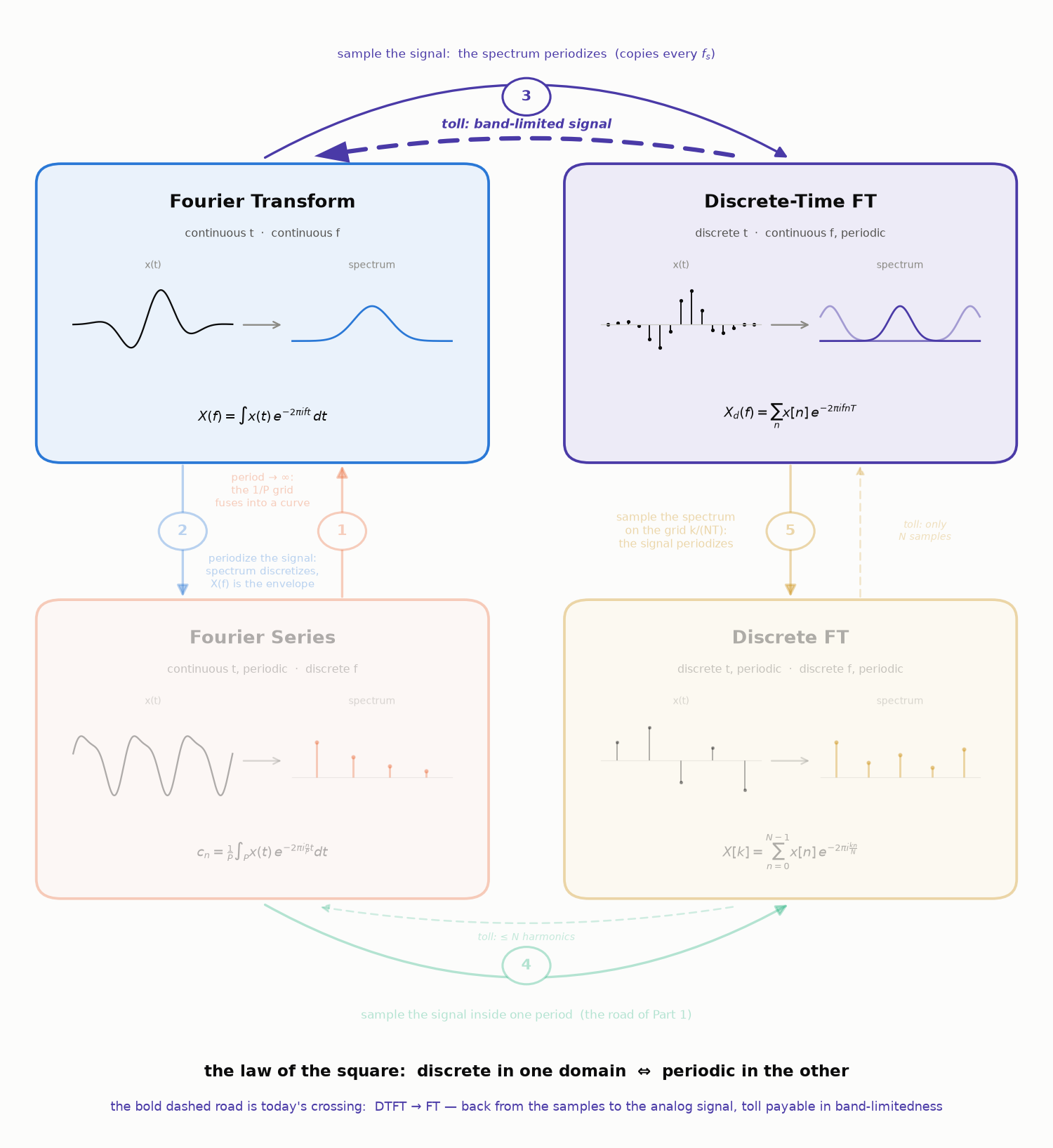
Here is today’s journey on the map of Four Shades. Of all the roads on it we are crossing the dashed one, in bold below — backwards along bridge three, from the sampled world to the analog one, paying the toll written on it:
What “band-limited” must mean
A signal is band-limited if its spectrum lives inside a finite window: there is a band edge $B$ with
$$ X(f) = 0 \quad \text{for all } |f| \ge B. $$In pictures this is row 1 of the copies figure below: the whole transform is a single hump that dies out completely before the edges of the picture — $X$ is identically zero outside a finite stretch of the frequency axis. Read physically: the signal contains no oscillation faster than $B$ hertz; above that frequency there is simply nothing to represent.
Two honest remarks before we lean on this definition. First, strictly band-limited signals are idealizations: Four Shades proved that a nonzero signal cannot be band-limited and time-limited at once, and every real recording ends — so no signal in practice satisfies the definition exactly. Second, engineering makes the definition true by force: before an ADC ever sees the signal, an analog anti-aliasing filter cuts away everything above a chosen band edge. For sound this costs nothing audible — the ear gives up near $20$ kHz anyway, so a filter parked just above that discards only what no listener could miss. (Hold that thought; it returns when we ask why CDs run at $44.1$ kHz.)
The theorem, stated
Theorem. Let $x$ be band-limited with band edge $B$, and sample it every $T$ seconds — a sampling rate of $f_s = \frac{1}{T}$. If
$$ f_s > 2B, $$then the samples $x(nT)$ determine the continuous signal completely: every value between the samples can be rebuilt, exactly, by the explicit formula $(\star)$ below.
Both landmarks of Part 2 reappear here with names attached: $2B$ — twice the band — is the Nyquist rate: sample faster than it, and the signal is exactly recoverable from the samples; sample at it or slower, and recovery is no longer guaranteed. From the sampler’s point of view, $\frac{f_s}{2}$ is the Nyquist frequency: the ceiling below which a signal’s spectrum must stay for a rate of $f_s$ to recover the signal. Note the inequality is strict: $f_s = 2B$ exactly is not enough, and a section below shows the counterexample where the boundary case fails.
The proof we already drew
Start from the identity that bridge three of Four Shades derived: sampling a signal every $T$ periodizes its spectrum,
$$ X_d(f) = \frac{1}{T} \sum_{m=-\infty}^{\infty} X(f - m f_s). $$Here $X(f)$ is the Fourier transform of the analog signal $x(t)$; $T$ is the sampling step and $f_s = \frac{1}{T}$ the sampling rate; $X_d(f) = \sum_n x(nT)\, e^{-2 \pi i f n T}$ is the DTFT — the spectrum computed from the samples alone; and each integer $m$ contributes one term $X(f - m f_s)$, a copy of the original spectrum slid $m$ grid steps along the frequency axis (the picture is the copies figure of Four Shades; today we need row 2 of it):
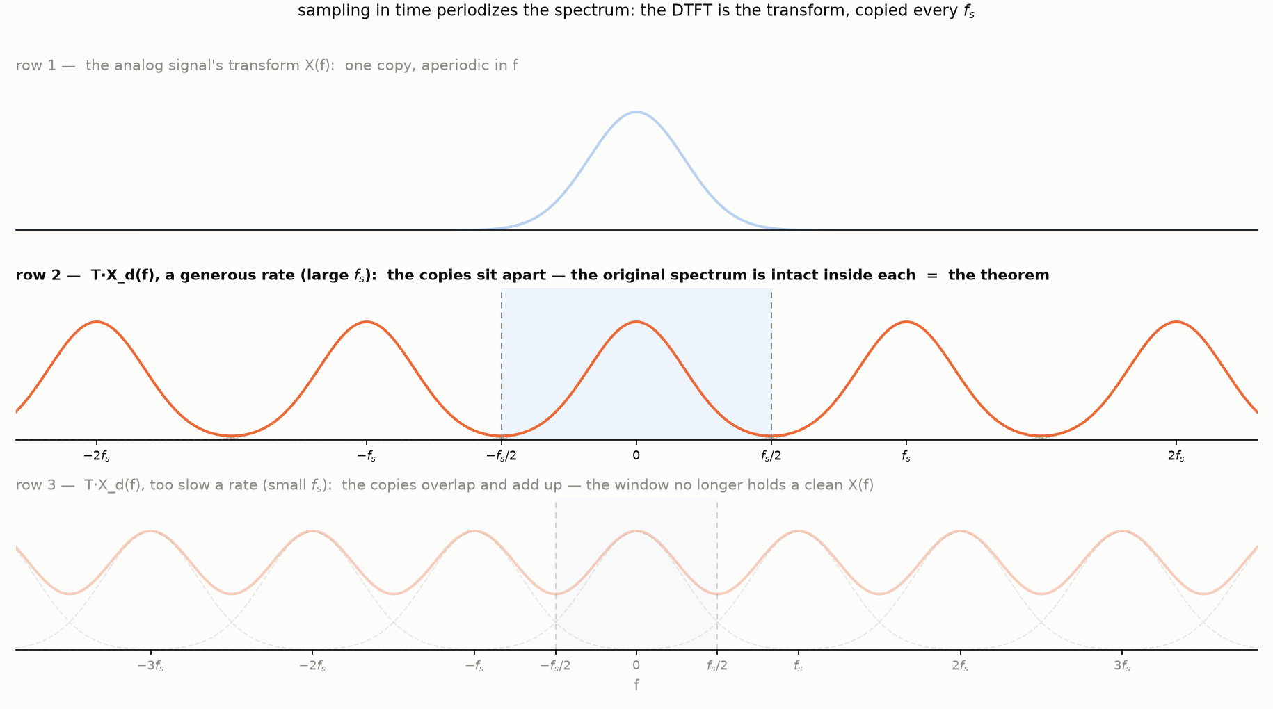
Now put the two hypotheses side by side. Each copy occupies $(-B, B)$ around its own center; the centers sit $f_s$ apart; and $f_s > 2B$ means the spacing exceeds the width. So the copies cannot touch — between consecutive copies there is a strip of silence, and the central period $\left( -\frac{f_s}{2}, \frac{f_s}{2} \right)$ contains exactly one thing: the original $X(f)$, intact. That is row 2 of the picture above, and that one bright row already contains the whole theorem: nothing about the analog signal was lost, because its entire transform sits undamaged inside the spectrum of the sampled one.
It remains to cut the copy out and turn it back into the signal. Multiply $X_d$ by the rectangular cutter
$$ H(f) = \begin{cases} T, & |f| \le \frac{f_s}{2}, \\ 0, & \text{otherwise} \end{cases} \;=\; T \cdot I_{[-f_s/2,\, f_s/2]}(f) $$— $T$ times the indicator of the central period ($I_A$ equals $1$ on the set $A$ and $0$ elsewhere); the factor is $T$ rather than $1$ so as to cancel the $\frac{1}{T}$ the copies formula carries:
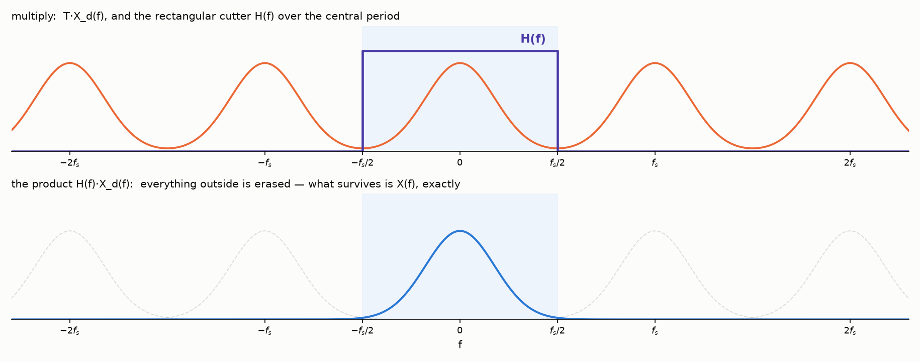
Everything outside the rectangle is erased, and the central copy survives untouched:
$$ \begin{aligned} H(f)\, X_d(f) &= T \cdot I_{[-f_s/2,\, f_s/2]}(f) \cdot \frac{1}{T} \sum_{m=-\infty}^{\infty} X(f - m f_s) \\ &= I_{[-f_s/2,\, f_s/2]}(f) \sum_{m=-\infty}^{\infty} X(f - m f_s) \;=\; X(f). \end{aligned} $$Now the Fourier integral rebuilds the signal from it:
$$ \begin{aligned} x(t) &= \int_{-\infty}^{\infty} X(f)\, e^{2 \pi i f t}\, df = \int_{-f_s/2}^{f_s/2} T\, X_d(f)\, e^{2 \pi i f t}\, df \\ &= \sum_{n=-\infty}^{\infty} x(nT) \int_{-f_s/2}^{f_s/2} T\, e^{2 \pi i f (t - nT)}\, df \end{aligned} $$— in the last step we substituted the DTFT sum $X_d(f) = \sum_n x(nT)\, e^{-2 \pi i f n T}$ and swapped the sum with the integral (the by-now-familiar juncture: honest for absolutely summable samples, by the same Weierstrass argument as in Four Shades). The remaining integral is an old friend: it is the rectangle-to-sinc computation from bridge two of Four Shades, run with the roles of time and frequency swapped. Writing $\tau = t - nT$:
$$ \begin{aligned} \int_{-f_s/2}^{f_s/2} T\, e^{2 \pi i f \tau}\, df &= T\, \frac{e^{\pi i f_s \tau} - e^{-\pi i f_s \tau}}{2 \pi i \tau} = T\, \frac{\sin(\pi f_s \tau)}{\pi \tau} \\ &= \frac{\sin(\pi f_s \tau)}{\pi f_s \tau} = \operatorname{sinc}(f_s \tau), \end{aligned} $$the sinc again — this time in the time domain, one bump per sample:
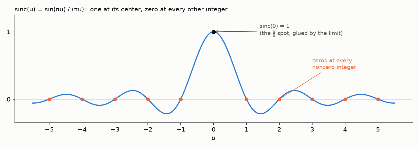
Put the pieces together:
$$ x(t) = \sum_{n=-\infty}^{\infty} x(nT)\, \operatorname{sinc}\!\left( \frac{t - nT}{T} \right). \tag{$\star$} $$This is the Whittaker–Shannon interpolation formula, and it deserves a slow read. Each sample $x(nT)$ launches its own sinc, centered at its own instant $nT$ and scaled to its own height. At the instant $t = mT$ the formula returns exactly $x(mT)$ — the $m$-th sinc equals $1$ at its center (at that one point its formula reads $\frac{0}{0}$, and the value $1$ is the classic limit $\frac{\sin u}{u} \to 1$ — the black dot in the picture above) while every other sinc is passing through one of its zeros, so no neighbor interferes:
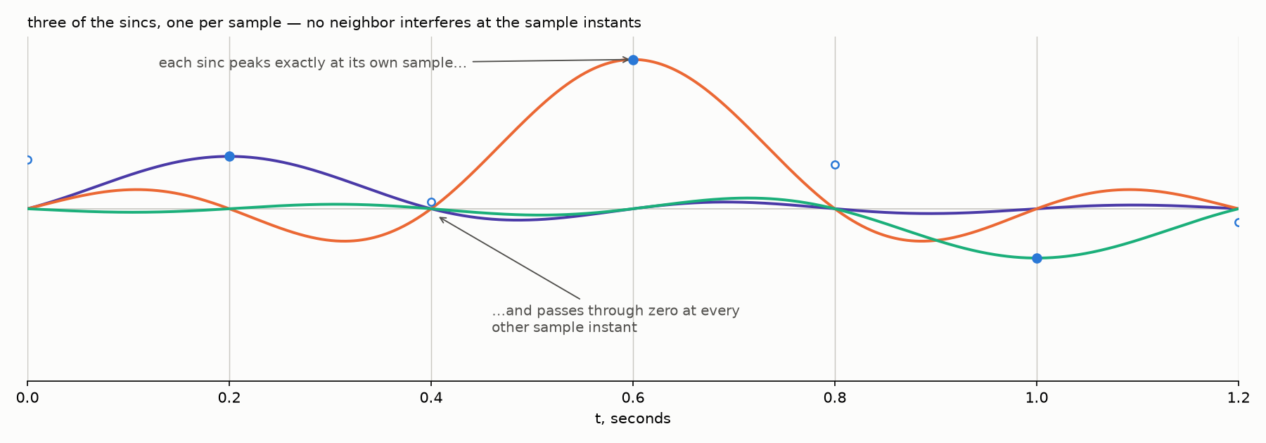 Between the instants, all the
sincs speak at once, and their sum fills in the continuous curve — the
values the recording never measured, restored by the theorem. This is
the third interpolation of our series, kin to two we have already met —
Part 2’s green
model
threading every sample, and the Dirichlet reconstruction of Four
Shades’ return roads.
Those two lived in periodic worlds with finitely many samples per
period; the sinc train is their full-line sibling — infinitely many
samples, no period, the entire time axis rebuilt.
Between the instants, all the
sincs speak at once, and their sum fills in the continuous curve — the
values the recording never measured, restored by the theorem. This is
the third interpolation of our series, kin to two we have already met —
Part 2’s green
model
threading every sample, and the Dirichlet reconstruction of Four
Shades’ return roads.
Those two lived in periodic worlds with finitely many samples per
period; the sinc train is their full-line sibling — infinitely many
samples, no period, the entire time axis rebuilt.
And here is the formula at work on a concrete signal — three sinusoids with band edge $B = 2$ Hz, sampled at $f_s = 5$ Hz, comfortably above the Nyquist rate $2B = 4$ Hz:
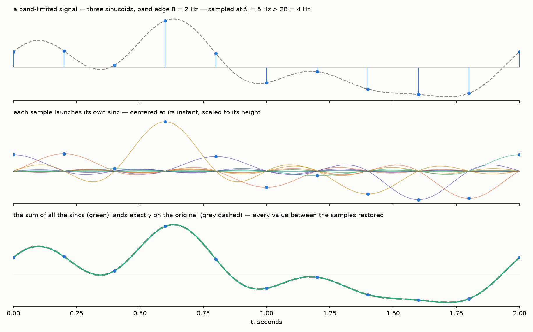
The middle row is the slow read made visible: one scaled sinc per sample, peaking at its own sample and silent at all the others. The bottom row is the theorem itself: the sum of the sincs lands exactly on the original — the green curve covers the grey dashed one entirely, every value between the samples included.
The boundary case bites
Why must the inequality be strict? Sample at the Nyquist rate exactly, $f_s = 2B$, and aim the sampler at the worst inhabitant of the band — a sine sitting right at the edge, $x(t) = \sin(2 \pi B t)$. The samples land at $t = \frac{n}{2B}$:
$$ x\!\left( \frac{n}{2B} \right) = \sin(\pi n) = 0 \qquad \text{for every integer } n. $$Every sample is zero — the sine is measured precisely at its zero crossings:
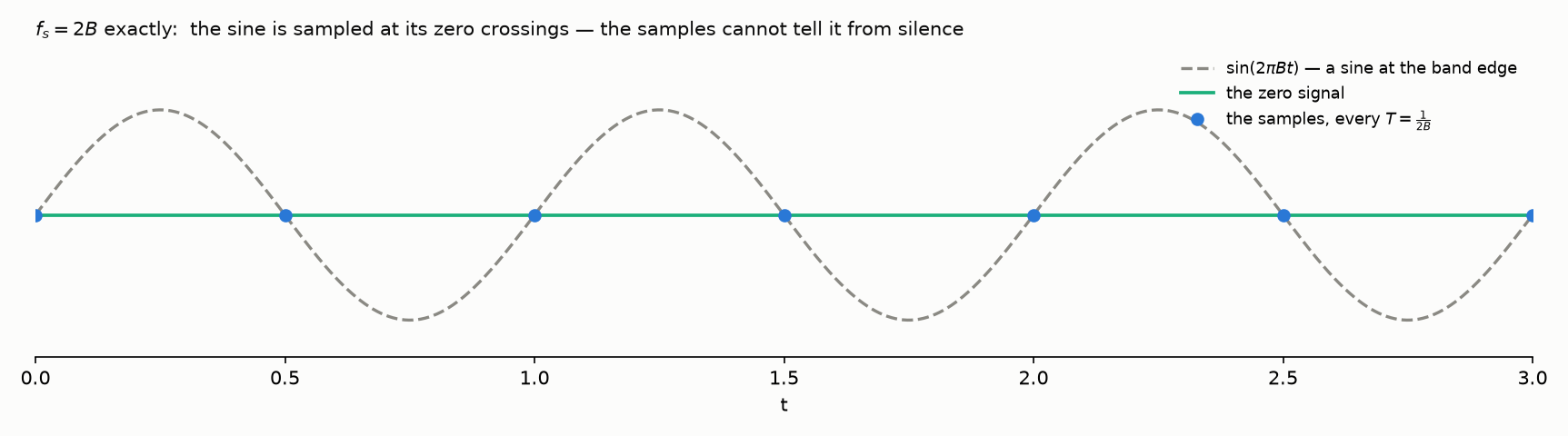
The recording is empty, indistinguishable from a recording of silence. Two different signals — the edge sine and the zero signal — pass through the same samples, so no formula, $(\star)$ or any other, can promise to restore “the” original: the information was lost at the sampling stage, before any reconstruction began.
The copies picture says the same thing in the frequency domain. At $f_s = 2B$ the neighboring copies do not overlap — but they touch: the edge of each copy lands exactly on the edge of the next. Our sine lives entirely on that shared edge, and its spectral spikes cancel against their mirror twins from the neighboring copy — the spectrum of the samples comes out identically zero, which is the frequency-domain face of the empty recording. Touching is already too much; hence the strict inequality.
Aliasing, or the wheels that spin backwards
Start from an identity that holds at any sampling rate: at the sample instants $t = nT$,
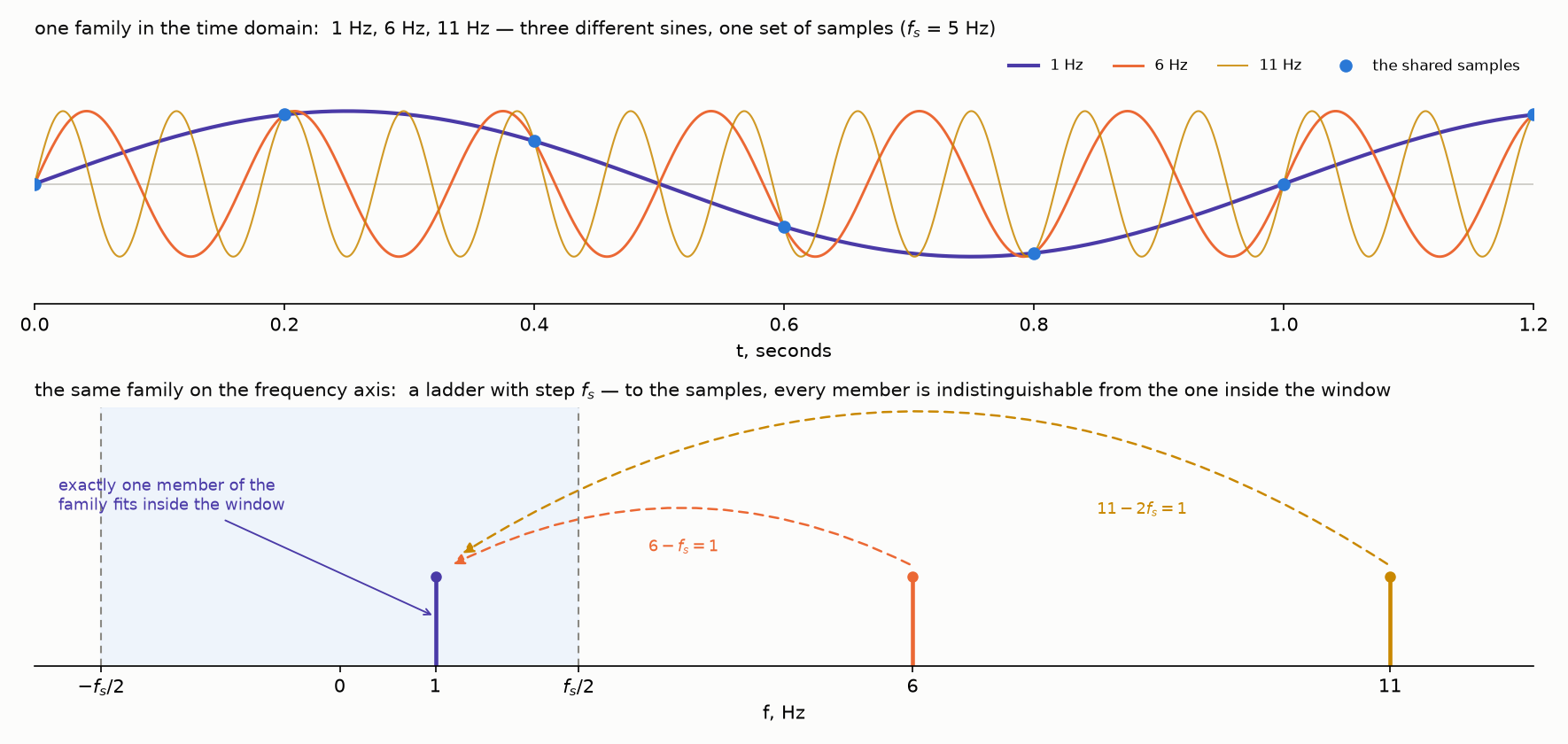
$$ e^{2 \pi i (f - f_s)\, n T} = e^{2 \pi i f n T} \cdot e^{-2 \pi i n} = e^{2 \pi i f n T}, $$so the frequencies $f$, $f \pm f_s$, $f \pm 2 f_s, \dots$ produce identical samples — sampling always confuses each such family of frequencies. The copies formula states the very same fact on the frequency axis: $X_d$ stacks the shifted copies $X(f - m f_s)$ on top of one another precisely because, to the samples, all the frequencies of one family are indistinguishable. The theorem’s hypothesis is what keeps the confusion harmless: exactly one member of every family fits inside the window $\left( -\frac{f_s}{2}, \frac{f_s}{2} \right)$. One always exists — subtract from any frequency the nearest multiple of $f_s$, and the remainder is at most $\frac{f_s}{2}$ away from zero — and two never fit at once, because distinct members sit at least $f_s$ apart while the window is only $f_s$ wide. For a signal band-limited below $\frac{f_s}{2}$ the in-window member is the true one — so picking the in-window candidate, which is all a reconstruction can ever do, picks correctly. Both halves of that story fit in one picture:
Now break the hypothesis: sample slower than the Nyquist rate, so that the copies overlap — row 3 of the copies picture, back on stage with today’s villain at full strength:
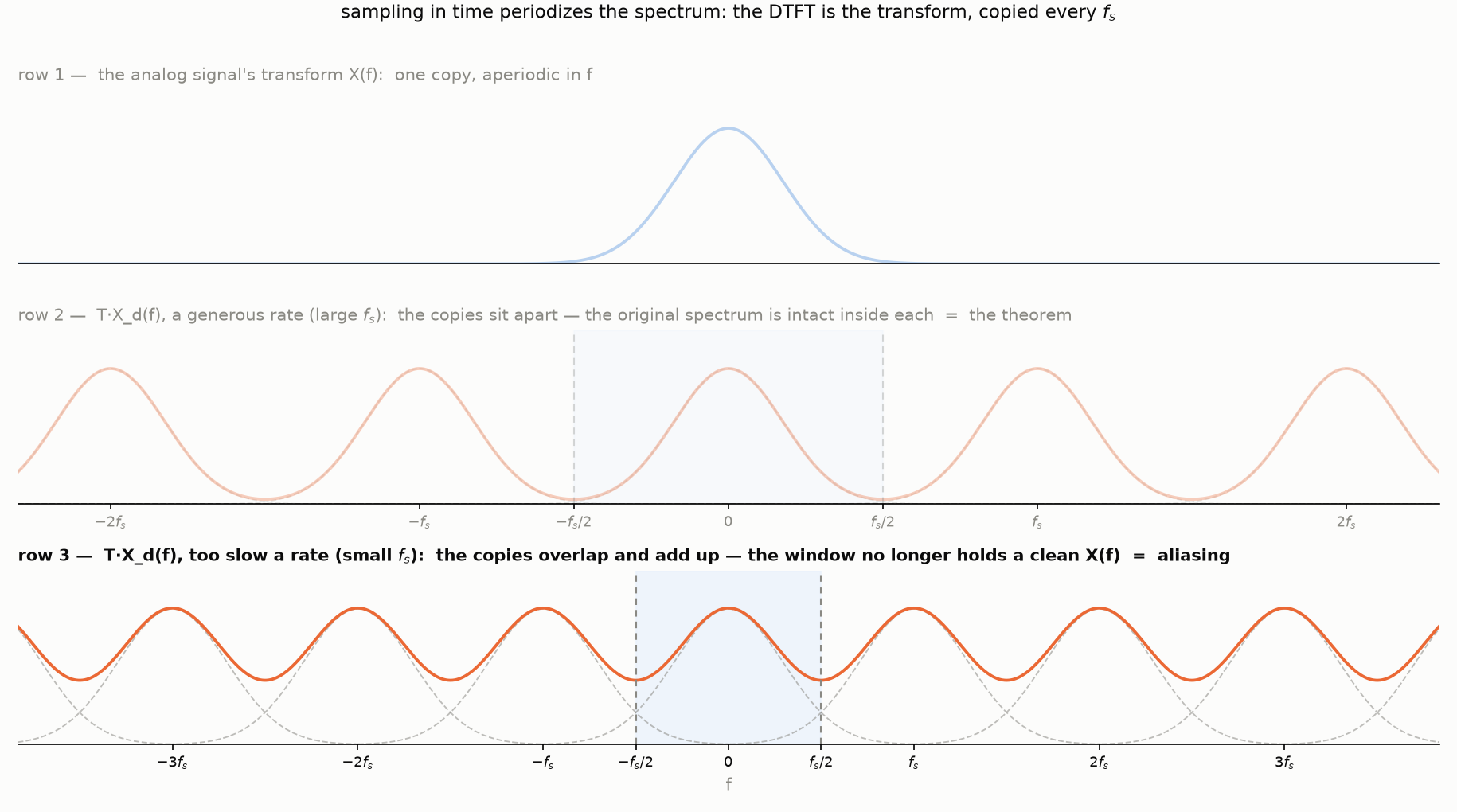
The true frequency is pushed outside the window, and the family member left inside is an impostor. Concretely: sample the $6$ Hz member of the family above at $f_s = 5$ Hz. The tone sits above $\frac{f_s}{2} = 2.5$ Hz, its in-window family member is $6 - 5 = 1$ Hz — and, as the family picture already showed, the samples of the $6$ Hz sine are exactly the samples of the $1$ Hz sine:
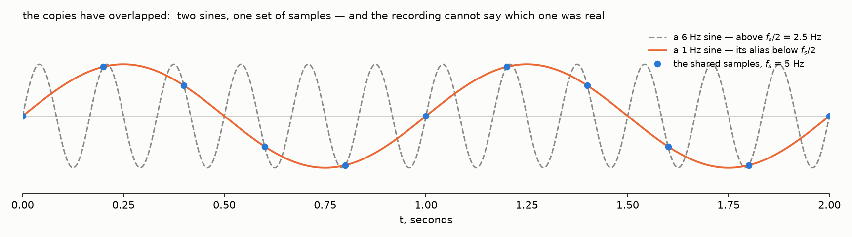
The recording cannot say which candidate was real, so a $6$ Hz tone goes in and a $1$ Hz impostor comes out. The impostor has a name — an alias — and the phenomenon is not exotic: you have watched it in every western. Film runs at $24$ frames per second — a sampler at $24$ Hz pointed at a stagecoach wheel. A wheel with $k$ spokes looks the same after $\frac{1}{k}$ of a turn, so the camera effectively watches a periodic pattern whose frequency is $k$ times the rotation rate — far above $12$ Hz for any wheel at speed. The pattern aliases. Spokes advancing slightly less than one full spoke-step per frame land, in every new frame, a little behind the previous frame’s spoke positions — and the eye reads a slow rotation backwards. Exactly one step per frame, and the wheel stands still under a galloping coach:
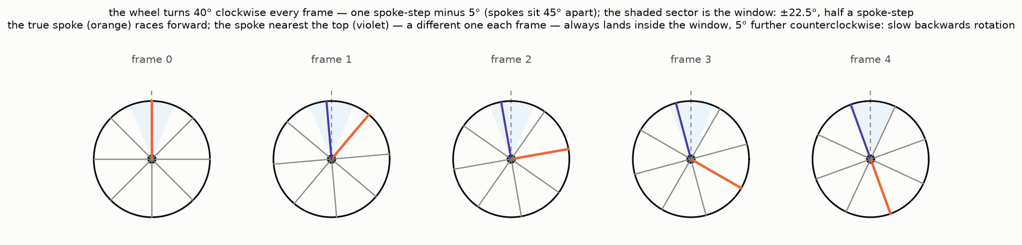
That is the wagon-wheel effect, and its kin are everywhere: a fan under a strobe light, the frozen propellers in phone videos of airplanes.
The dictionary between the wheel and the theorem is short. Film is sampling: one frame — one sample, so let us measure frequencies per frame; then the sampling rate is $f_s = 1$ by definition, and the window $\left( -\frac{f_s}{2}, \frac{f_s}{2} \right)$ is $\left( -\frac{1}{2}, \frac{1}{2} \right)$. The signal is the spoke pattern, and its natural unit is the spoke-step: one pattern-period = one spoke-step = $45°$. In the frames above the wheel turns $40°$ per frame, so the true frequency is $f_0 = \frac{40}{45} = \frac{8}{9}$ of a period per frame — outside the window: the hypothesis $f_0 \lt \frac{1}{2}$ is broken. (It is broken for any real wheel at speed — spokes sweep past far more often than twelve times a second, half of film’s $24$.) The window converts into the shaded sector, $\pm \frac{45°}{2} = \pm 22.5°$; the in-window family member, $\frac{8}{9} - 1 = -\frac{1}{9}$ of a period, is $-5°$ per frame — the slow backwards drift, this time computed rather than observed. (For a rotating pattern a negative frequency simply means turning the other way.)
And here is what an honest frame rate looks like. Give the film eight times the frames, so the wheel turns only $5°$ per true frame — safely inside the window — and the illusion evaporates:
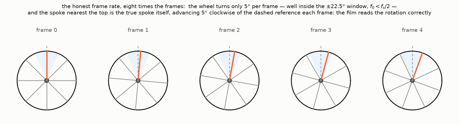
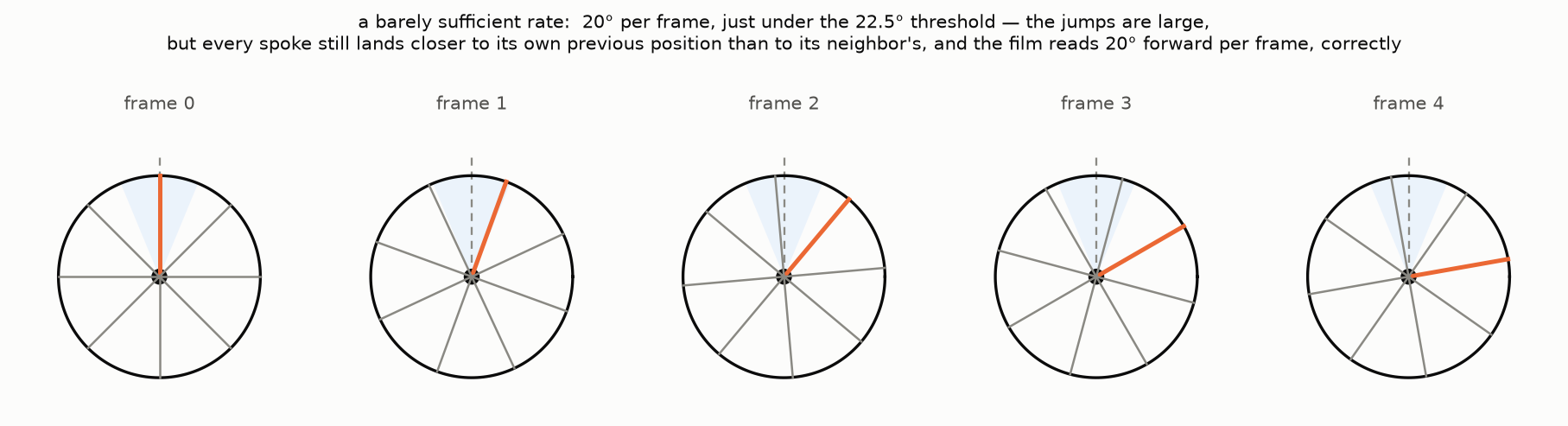
Eight times is comfort, not necessity: any rate that keeps the turn per frame under half a spoke-step — any $f_s > 2 f_0$ — is honest. Here is a barely sufficient one, $20°$ per frame, just under the threshold. The jumps are large, but from each frame to the next every spoke still lands closer to its own previous position than to its neighbor’s — and that is the real criterion: the eye pairs each spoke with the nearest spoke of the previous frame, and sampling is honest exactly when this pairing is the true one:
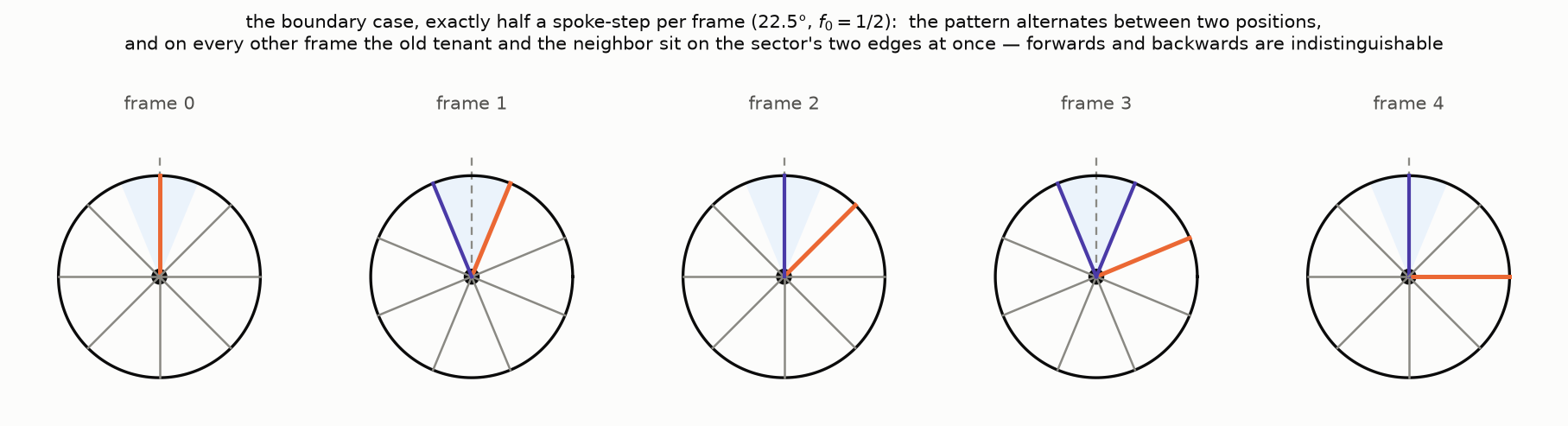
Push to the threshold itself — exactly half a spoke-step per frame, $f_0 = \frac{1}{2}$ — and the pairing becomes a coin toss: each spoke lands exactly halfway between two old positions, the pattern merely alternates, and forwards is indistinguishable from backwards — the wheel-world twin of the edge sine sampled at its zero crossings:
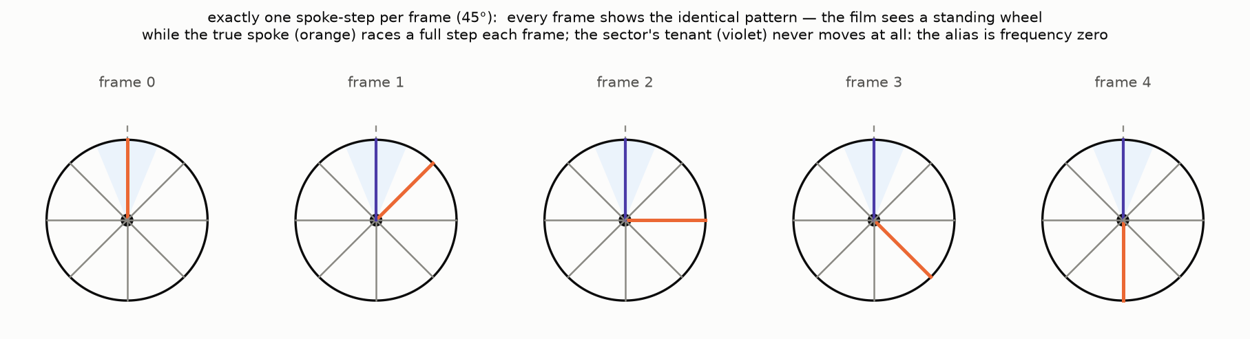
Past the threshold the pairing goes wrong — that is our first strip, $40°$ per frame read as $5°$ backwards. And one speed deserves its own portrait — the illusion’s fixed point. At exactly one full spoke-step per frame every spoke lands precisely on its neighbor’s old position — every frame is identical, and the film sees a standing wheel under a galloping coach, the alias at frequency zero. A shade slower and the wheel crawls backwards; a shade faster, forwards: the whole cycle repeats every spoke-step:
The threat of aliasing also explains a famous number. Human hearing ends near $20$ kHz, so audio needs $f_s > 40$ kHz — and CDs run at $44.1$ kHz. The extra $4.1$ kHz is working room for the anti-aliasing filter: an analog low-pass cannot cut off instantly, so it passes everything up to $20$ kHz and fades to silence across the $20$–$22.05$ kHz gap — and whatever survives in that gap is harmless, being both inaudible and below $\frac{f_s}{2}$. (Why $44100$ and not a round $44000$? A relic: early digital audio was stored on video recorders, and $44100$ samples per second is what fits as three samples per line on both TV standards of the era.)
Three names, four people
The theorem’s name depends on where you learned it, and every version is defensible. Harry Nyquist (1928) studied telegraphy and showed that a channel of band $B$ carries at most $2B$ independent pulses per second — the critical rate is rightly his, though he never stated the reconstruction theorem. E. T. Whittaker (1915) had already built the sinc series $(\star)$ as pure interpolation mathematics, with no signals in sight. Vladimir Kotelnikov (1933) was the first to state and prove the sampling theorem as an engineering fact — in a Soviet radio-engineering conference paper that the West did not read for decades. And Claude Shannon (1949) proved it again as a foundation stone of information theory, and it entered the world’s textbooks under his name. So the Russian literature says Kotelnikov’s theorem, the Western says Nyquist–Shannon, mathematicians remember Whittaker’s cardinal series — three names, four people, one road across the map.
Onward
With this post the Fourier road of the blog closes its loop. The trilogy built the discrete world from sound up; Four Shades drew the map and its law; today the dashed road home is paved — samples back to the analog signal, toll checked at the gate. The debts are settled.
The blog’s next journey is quantum mechanics — a change of subject on the surface, and secretly a continuation. In quantum mechanics a particle’s position and momentum descriptions are a Fourier pair — the momentum wavefunction is the Fourier transform of the position one — and the uncertainty principle is Part 3’s time–frequency trade-off wearing a lab coat: a signal cannot be narrow in time and in frequency at once, and a particle cannot be sharp in position and in momentum at once — for exactly the same mathematical reason. The map stays open; the roads keep going. See you in the quantum world.