From the Fourier Series to the Spectrogram, Part 2: Reading the DFT

Part 1 ended with the machinery built. The Discrete Fourier Transform takes the $N$ samples of a recording and returns $N$ complex numbers:

$$ X[k] = \sum_{n=0}^{N-1} x[n]\, e^{-2 \pi i \frac{k n}{N}}, \qquad k = 0, 1, \dots, N-1. $$

$N$ numbers in, $N$ numbers out — and every trace of physical time gone: the formula sees only the two integers $k$ and $n$. That was a feature during the derivation, but it leaves us unable to answer the simplest practical question. Remember the hum? Back in Part 1, arguing that the frequency view is worth having, we took a recording polluted by the 50 Hz buzz of the power line — hopeless to fix in the time domain, where the hum is smeared over every sample — and fixed it in the frequency domain, where the hum is a single column: transform, erase that column, transform back, and the melody survives while the buzz is gone. A fine trick — except that now, with the transform actually in our hands, try to perform it. Which column? Which $k$ is 50 Hz? This part is about learning to read the DFT’s output: matching indices to physical frequencies, seeing what the resolution of that matching costs, and discovering along the way why half of the output is a mirror image of the other half.

What does X[k] measure?

Look at the DFT formula through the lens of the inner product from Part 1’s sifting-property proof. There we needed it for continuous signals: multiply pointwise, then integrate — the integral standing in for “add everything up” over a continuum. For finite lists of samples the same recipe is simpler still: multiply pointwise and literally add. That is the ordinary dot product of vectors — the very case the notation was borrowed from in the first place — plus one refinement for complex signals: the second factor gets conjugated (that is what the overline over $w_k[n]$ denotes):

$$ X[k] = \sum_{n=0}^{N-1} x[n]\, \overline{w_k[n]} = \langle x, w_k \rangle, \qquad w_k[n] = e^{2 \pi i \frac{k n}{N}}. $$

Each coefficient is the inner product of the signal with one basis oscillation $w_k$ — a number that measures how much the signal resembles that oscillation, exactly like a dot product measures how much one vector leans along another. As $n$ runs through the $N$ samples, the exponent of $w_k$ grows to $2 \pi i k$: the basis oscillation makes exactly $k$ full turns across the recording — Part 1’s “only oscillations that fit a whole number of times into the period” rule, wearing its discrete clothes. Here is the whole cast at once, drawn over one window of $N = 8$ samples:

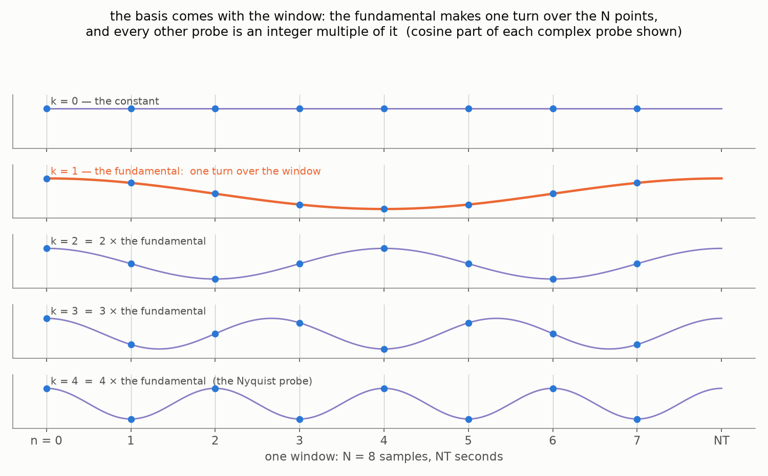
This picture is worth pausing on, because it shows what dictates the basis: nothing but $N$ itself. Fix the window — $N$ samples, $NT$ seconds — and the slowest nonzero probe is forced: one full turn over exactly those samples, frequency $1/(NT)$. The rest of the vocabulary follows automatically, because every other probe is an integer multiple of that fundamental — two turns, three turns, up the ladder. Choose the window and the basis comes with it; the DFT then offers its $N$ probe frequencies — zero turns, one turn, two turns, … — and reports the signal’s resemblance to each.

(A detail worth a second look: in the picture, the curves run past the last sample, all the way to $t = NT$. That is not sloppiness — the window genuinely lasts $NT$ seconds: $N$ intervals of $T$ each, with a sample at the start of every interval. The last sample therefore sits at $n = N - 1$, while $t = NT$ is where the next period would begin — and a whole-turn probe arrives there exactly as it started. That endpoint belongs to the copy, not to this window; if we also sampled at $t = NT$, we would be counting the same point twice.)

These $N$ oscillations deserve a name, because they are more than measuring sticks: look back at the inverse DFT formula from Part 1 — it is $x[n] = \frac{1}{N} \sum_k X[k]\, w_k[n]$, the signal reassembled as a weighted sum of these very oscillations. So the set $w_0, \dots, w_{N-1}$ is everything the DFT can say: the forward transform measures how much of each word the signal contains, the inverse composes the signal back out of the words. We will call this set the DFT’s vocabulary — $N$ words, and nothing in between.

Here is what the probes look like in the flesh — the beginning of the vocabulary, drawn over the same sampled signal for four different recording lengths:

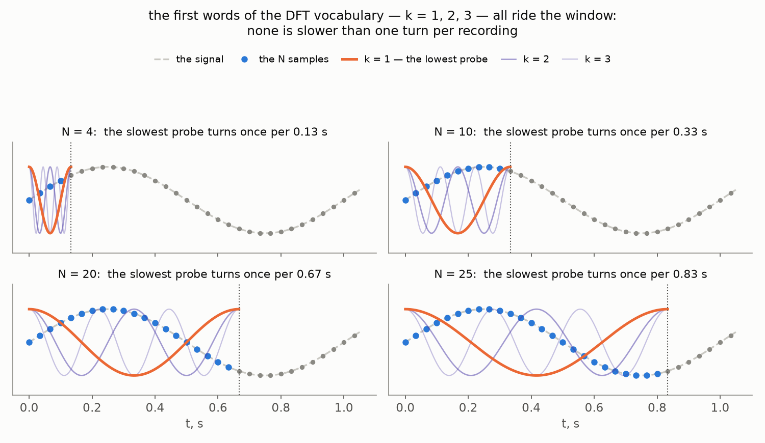
In every panel the bold orange curve is the $k = 1$ probe — the lowest oscillating frequency the basis has; the fainter curves behind it are $k = 2$ and $k = 3$, twice and three times faster. One full turn per recording, whatever the recording turns out to be — and that is worth staring at while $N$ is small. At $N = 4$ even the slowest word in the vocabulary races through its full turn before the signal has done anything at all: every probe the DFT owns is far too fast for this signal, and a good description is simply not on offer. Only as the recording grows does the vocabulary reach down to where the signal actually lives — by $N = 25$ the lowest probe finally oscillates at almost the signal’s own pace.

(Keep one thing in mind while looking at these curves: they are drawn at phase zero, every one starting from its peak. In the true approximation each probe will additionally come with its own phase shift — the weights the DFT assigns are complex numbers, and a complex weight slides its probe in time. How exactly that works — and how peak-started cosines manage to assemble a zero-started signal — is a couple of pictures away.)

And what does the vocabulary say, once every word gets its weight? Sum all $N$ probes with the coefficients the DFT assigns them — that is exactly the inverse DFT — and draw the sum as a continuous curve. This is the signal the DFT actually believes in:

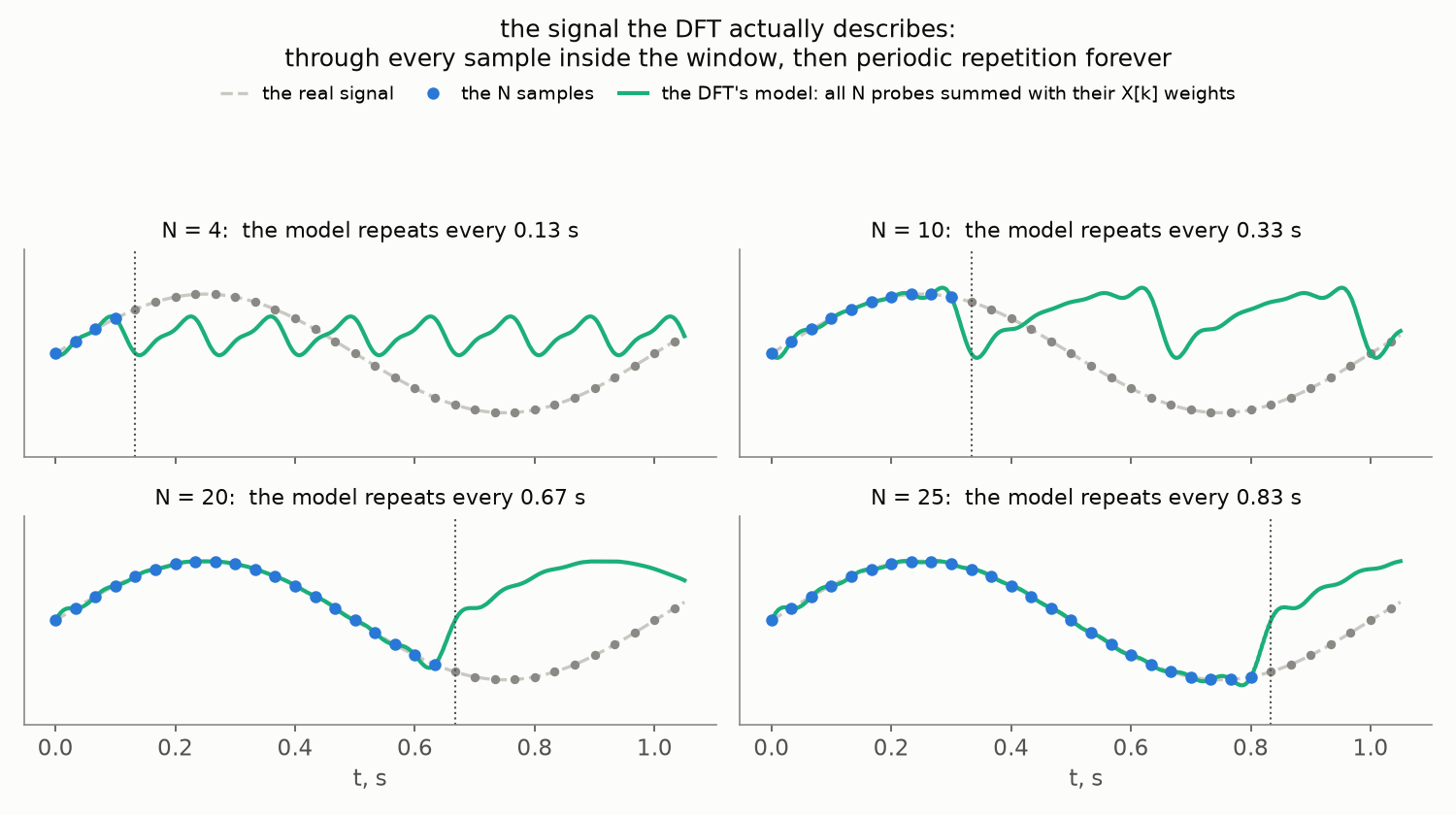
Two things to see here. Inside the window, the green model passes through every blue sample exactly — $N$ numbers in, $N$ numbers out, the books balance as always.

(Why exactly, and not merely very closely? That has a beautiful answer, but it deserves its own stretch of road — and gets one: the appendix at the end of the post, for whenever the linear-algebra mood strikes.)

💡 Wait — how do cosines add up to a sine? Every probe we drew starts at its peak, yet the green model starts wherever the signal starts — at zero, even. The resolving detail is that the weights $X[k]$ are complex: each carries a magnitude and a phase, and a complex weight shifts its probe in time. Pair each $k$ with its mirror twin $N - k$, and their joint contribution to the model is $\tfrac{2 |X[k]|}{N} \cos\!\big( 2 \pi \tfrac{k}{NT}\, t + \arg X[k] \big)$ — a cosine nudged to its own starting point, Part 1’s $A \cos(\dots - \phi)$ story again. The pictures draw every probe at phase zero; the sum deploys each one shifted, with the $k = 0$ word — the plain mean — soaking up any constant offset. A sine is merely a cosine whose phase is nudged by a quarter turn.

Outside the window, the model does the only thing a sum of whole-turn oscillations can do: repeats, with the window’s own period. The DFT never models your signal as it is — it models a periodic world assembled from your window, Part 1’s glued copies meeting us yet again. At $N = 4$ that world has almost nothing to do with the real signal; by $N = 25$ it is a faithful model of the window — and still a pure invention everywhere else. (This picture was suggested by a friend of the blog — thank you!)

Zoom out, and the same experiment shows when the invention comes true. Everything depends on how the window relates to the signal’s own period:

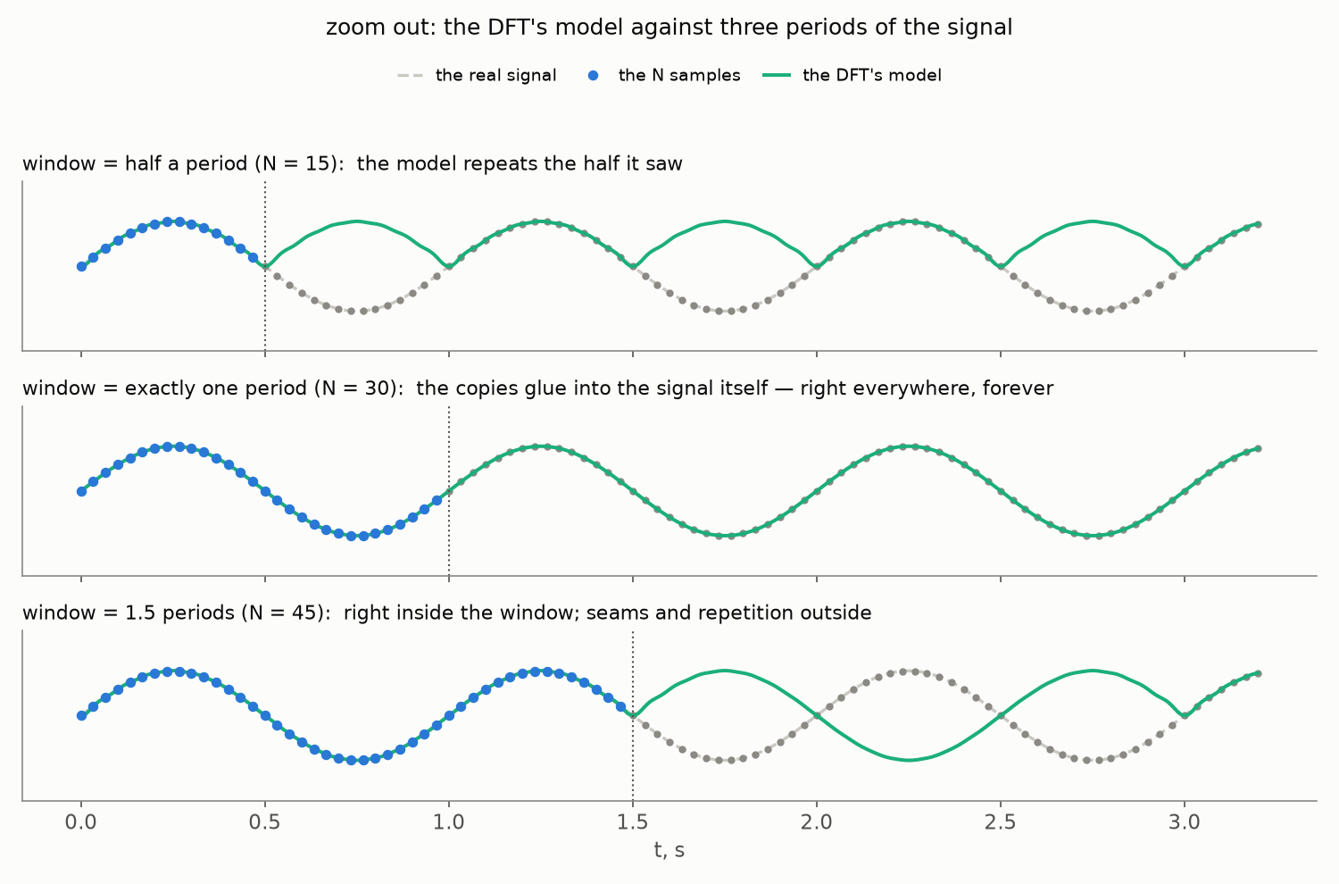
The middle panel is the special one. When the window holds exactly one period of the signal (or any whole number of them), the glued copies reproduce the signal — the model is correct not only inside the window but everywhere, forever. That is the DFT at its happiest: the signal’s frequency coincides with one of the probes. In the other two panels the window holds half a period and one and a half: the model still passes through every sample it saw, but its periodic continuation has nothing to do with the real signal — the top one never even goes negative, the bottom one continues in counter-phase — and at every seam the curve kinks. Those kinks have a price in the spectrum, and Part 3 charges it under the name spectral leakage.

Turn the “whole turns” rule around, and it becomes a restriction important enough to put in bold: whole numbers of turns are all the DFT has. Its basis contains the constant ($k = 0$) and the oscillations that fit a whole number of times into the recording — nothing else. A tone that completes, say, two and a half turns over our $N$ samples is simply not in the vocabulary: no single $X[k]$ is “its” coefficient. Real recordings contain such tones all the time, of course, and the DFT must express them somehow — smearing them across the whole-turn vocabulary it does have. The consequences of that smearing (it goes by the name spectral leakage) will matter a great deal when we build the spectrogram in Part 3; for now, keep in mind that the DFT’s world is quantized to whole turns.

💡 The $k = 0$ probe makes zero turns: $w_0[n] \equiv 1$, and $X[0] = \sum_n x[n]$ is just $N$ times the average of the signal. Audio engineers call it the DC component (from “direct current” — the electrical origin shows). For sound it is normally near zero: pressure oscillates around the atmospheric baseline, and the microphone measures only the deviation.

From the index to hertz

So $X[k]$ measures the content of “$k$ turns per recording”. To turn that into hertz, bring back the physical time that the DFT so pointedly forgot. The $n$-th sample was taken at $t = nT$, and the whole recording lasts $NT$ seconds — so “$k$ full turns per recording” is the physical frequency

$$ f_k = \frac{k}{NT} = k \frac{f_s}{N}, $$

where $f_s = 1/T$ is the sampling rate. The probe frequencies are not arbitrary: they form a uniform grid with step

$$ \Delta f = \frac{f_s}{N} = \frac{1}{NT}, $$

called the frequency resolution — no probe exists between $f_k$ and $f_{k+1}$, so the DFT simply cannot distinguish frequencies closer together than $\Delta f$.

Now, a question worth pausing on. The sampling rate is not really ours to choose — it is a property of the microphone and the ADC, fixed in hardware. The one knob we do control is $N$: how many samples we feed the transform. What exactly does that knob turn? Look again at the probe picture in the previous section — it holds the answer.

The basis rides the window, not the clock: more samples at the same rate means a longer recording, and the one turn of $w_1$ spreads over it. Write $w_1$ out and walk it back from the index notation to physical time, exactly the way we did for a general $k$:

$$ w_1[n] = e^{2 \pi i \frac{n}{N}} = e^{2 \pi i \frac{1}{NT} \cdot nT} $$

— the right-hand form is a sinusoid of physical frequency $\frac{1}{NT}$, caught at the moments $t = nT$. The $N$ sits in the denominator of the frequency: lengthen the recording, and the slowest probe slows down with it — $\Delta f = \frac{1}{NT}$ drops. And since every other probe sits at a multiple of it, the whole frequency grid tightens:

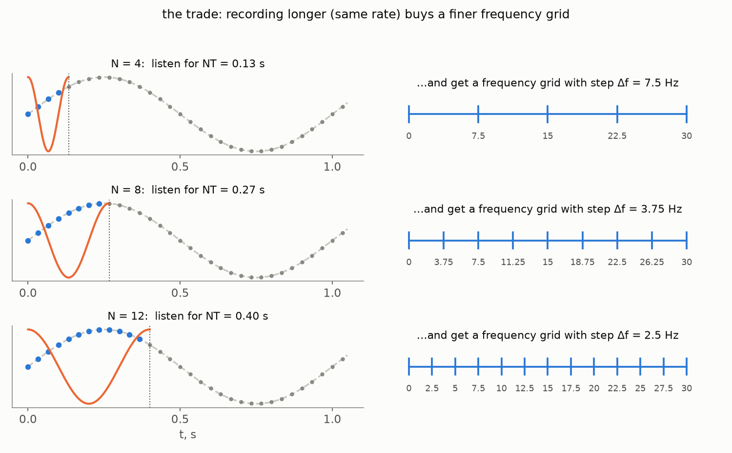
That is what the knob turns. Look at the second formula for $\Delta f$ again: $NT$ is simply the duration of the recording, so

$\Delta f = \dfrac{1}{\text{duration}}$ — frequency resolution is one over the listening time.

To tell two tones one hertz apart, you must listen for at least a second — only then does the slower tone fall a full turn behind and the difference become visible. There is no way around this trade, only a choice along it: this very tension — resolution in frequency versus locality in time — will return as the central design decision of the spectrogram in Part 3.

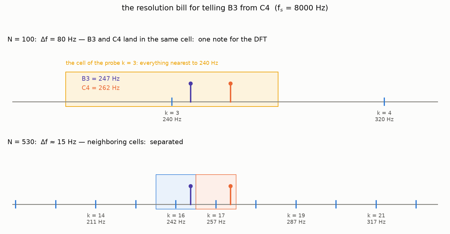
A worked example in unforgiving numbers: at $f_s = 8000$ Hz, taking $N = 100$ samples (an eighth of a second) gives $\Delta f = 8000 / 100 = 80$ Hz. That grid is too coarse to tell middle C (262 Hz) from the B just below it (247 Hz): both land in bin $k = 3$. To separate them you need $\Delta f$ around their 15 Hz gap — that is $N \approx 530$ samples, a fifteenth of a second. Music transcription from spectra is possible, but the resolution bill must be paid first. (A caveat for the careful: $\Delta f$ equal to the gap is the bare threshold — at that margin the two peaks only just stand apart, as the companion notebook at the end of this post shows; comfortable separation wants a finer grid still.)

The spectrum, at last

We can now do properly what Part 1 could only preview: plot the magnitudes $|X[k]|$ against their physical frequencies $f_k$. This picture is the (magnitude) spectrum of the recording:

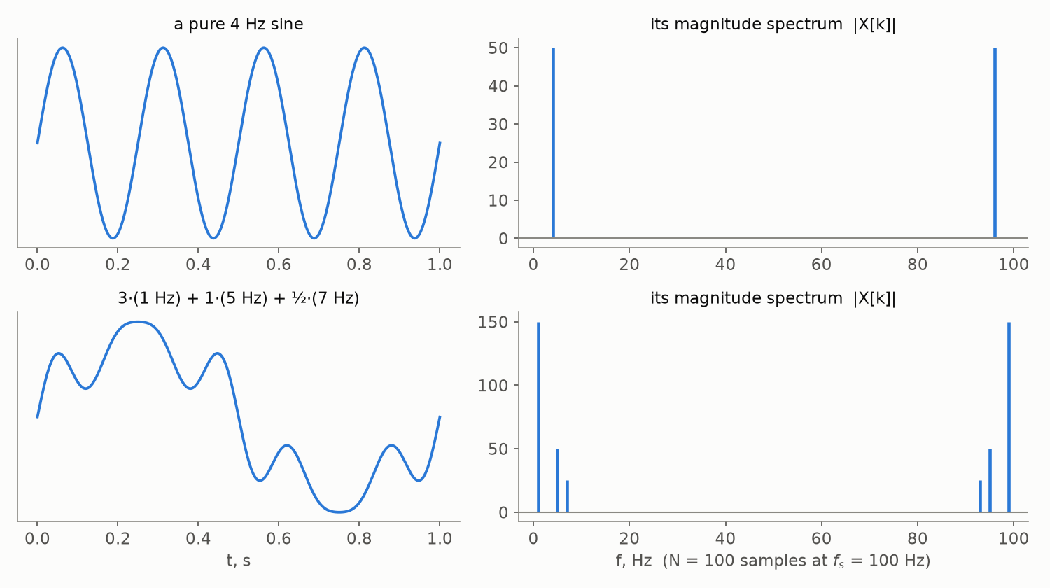
A pure sine shows up as a sharp spike at its frequency — plus a curious twin at the far end of the axis (explained below, in The mirror) — and a mix of three sines as three spikes with the right heights (and three twins), each component recoverable at a glance. This is the “hundreds of numbers → three meaningful ones” compression promised at the very start of Part 1 — delivered.

What about the other half of the complex number? Write $X[k]$ in polar form — every complex number is a length times a direction:

$$ X[k] = |X[k]|\, e^{i \varphi_k}, \qquad \varphi_k = \arg X[k]. $$

The length $|X[k]|$ is the magnitude we have just been plotting; the angle $\varphi_k$ is the phase, and it stores where in its cycle the $k$-th oscillation starts — Part 1’s $\phi_n$, one per harmonic. Much of speech processing works with magnitudes alone: what a vowel sounds like, which note was played, whether the hum is there — all of it lives in the magnitudes. The phase becomes essential the moment you need to rebuild the waveform — shifting every component back to its proper starting point — which is why speech synthesis and enhancement systems must treat it with care while a speech recognizer can throw it away.

The mirror

Look at the spectra again: the single 4 Hz sine lights up its own bin and a twin at 96 Hz, and in the three-sine mix the whole right half of the axis mirrors the left. This is not an artifact of the example — it is a theorem about every real-valued signal, and it takes four lines to prove. Compute the coefficient at index $N - k$ (the overline here and below is complex conjugation, $\overline{a + bi} = a - bi$ — the flip of the imaginary part’s sign):

$$ \begin{aligned} X[N-k] &= \sum_{n=0}^{N-1} x[n]\, e^{-2 \pi i \frac{(N-k) n}{N}} \\ &= \sum_{n=0}^{N-1} x[n]\, e^{-2 \pi i n}\, e^{2 \pi i \frac{k n}{N}} \\ &= \sum_{n=0}^{N-1} x[n]\, e^{2 \pi i \frac{k n}{N}} \\ &= \overline{\sum_{n=0}^{N-1} x[n]\, e^{-2 \pi i \frac{k n}{N}}} = \overline{X[k]}. \end{aligned} $$

One move per line. First, split the exponent: $\frac{N-k}{N} = 1 - \frac{k}{N}$, so the exponential factors into $e^{-2 \pi i n} \cdot e^{2 \pi i \frac{k n}{N}}$. Second, $e^{-2 \pi i n} = 1$ because $n$ is an integer — the same “signal lives on a grid” card we played to prove $c_{k+N} = c_k$ in Part 1. Third, recognize a conjugate: flipping the sign of the exponent conjugates each exponential, and the samples $x[n]$ are real — conjugation passes through them untouched — so the conjugation bar slides over the entire sum, and the sum under the bar is exactly the DFT formula for $X[k]$.

The second half of the spectrum is therefore the complex conjugate of the first, read backwards — and conjugation does not change magnitudes: $|X[N-k]| = |X[k]|$. Every spike below the middle has a twin above it, and the magnitude spectrum of any real signal is symmetric about $k = N/2$.

We have met this mirror before. Part 1’s exponential form split every real oscillation into a forward- and a backward-rotating exponential, with $c_{-n} = \overline{c_n}$ — and we promised the symmetry would resurface in the DFT. Here it is: by the periodicity $c_{k+N} = c_k$ that we proved when deriving the DFT, the coefficient $c_{-k}$ is $c_{N-k}$. The upper half of the DFT output is precisely the negative-frequency half of the spectrum, wrapped around by periodicity into the range $k = N/2, \dots, N-1$. The twin spike at “96 Hz” is really the spike at $-4$ Hz, filed under an alias.

💡 Do the books still balance? If half of the output mirrors the other half, doesn’t the DFT return only $N/2$ numbers’ worth of information for $N$ numbers of input? Count the real degrees of freedom (say $N$ is even). $X[0]$ is a sum of real samples — real, one number. $X[N/2]$ pairs with itself in the mirror ($N - N/2 = N/2$), forcing $X[N/2] = \overline{X[N/2]}$ — real, one number. The remaining $N - 2$ coefficients come in conjugate pairs, each pair carrying one independent complex number — two real ones. Total: $1 + 1 + \frac{N-2}{2} \cdot 2 = N$ real numbers. Exactly the information content of $N$ real samples — the books balance to the cent, as they must for an invertible transform.

The Nyquist frequency

The mirror axis itself deserves a name. The probe at the fold, $k = N/2$, is the oscillation

$$ w_{N/2}[n] = e^{2 \pi i \frac{(N/2) n}{N}} = e^{\pi i n} = (-1)^n $$

— the sequence $+1, -1, +1, -1, \dots$, flipping sign at every single sample. No oscillation representable on the grid can flip faster: there is nothing between the samples to flip in. Its physical frequency comes from the bin-to-hertz formula $f_k = k \frac{f_s}{N}$ of the resolution section, with $k = N/2$ plugged in:

$$ f_{N/2} = \frac{N}{2} \cdot \frac{f_s}{N} = \frac{f_s}{2}, $$

is the Nyquist frequency — the ceiling of what a given sampling rate can represent, sitting always at exactly half of it. Draw this axis onto the spectra from earlier, and the symmetry becomes something you can fold with your eyes:

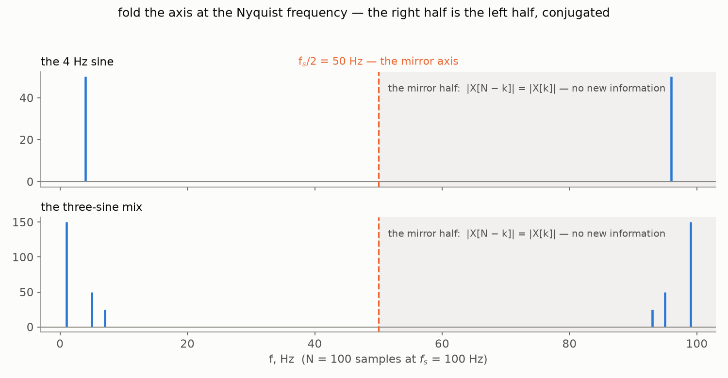
Everything above the ceiling and below $f_s$ is the mirror land we mapped in the previous section — present in the numbers, but carrying nothing new for a real signal. So here is the full geography of the DFT’s frequency axis on one picture:

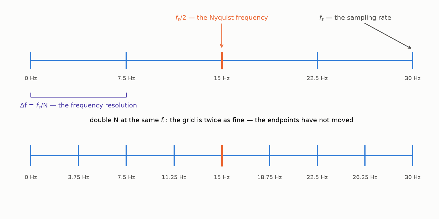
The genuinely informative range runs from $0$ to $f_s/2$ — which finally explains a number from Part 1: CD audio samples at 44.1 kHz because its ceiling must clear the ~20 kHz limit of human hearing, with a little engineering margin on top.

In fact, the ceiling is the visible edge of one of the most celebrated results in all of signal processing — and we finally know enough to state it properly:

The sampling theorem (Kotelnikov, 1933; independently Shannon, 1949; the frequency bears Nyquist’s name — this theorem was discovered by everyone). A continuous signal containing no frequencies higher than $f$ Hz is completely determined by its samples taken $f_s = 2f$ times per second.

Read the claim slowly, because it is startling. Between two neighboring samples, a continuous signal could seemingly wiggle any way it pleases — and the theorem says a band-limited one cannot: the samples pin down the entire continuous curve, exactly, nothing lost. This is the license behind everything we have done since Part 1 — the reason a list of numbers can honestly stand in for a sound wave, provided the wave had nothing above $f_s/2$ to begin with.

And if it did? The ceiling is a statement about what the grid can represent — but the analog world does not consult our grid. Frequencies above $f_s/2$ do not politely disappear at sampling; they fold back into the visible range under false names — aliasing, the theorem’s dark twin. The proof of the theorem, the folded world of aliasing, and even the fine print hiding in the statement above (sticklers: a sinusoid at exactly $f$ needs care) are a story for later in this Fourier journey — the theorem with three names (Kotelnikov, Shannon, Nyquist) will get a post of its own, and by then the machinery we keep building will have turned its proof into a single picture. Consider it teased.

Onward

We can now read a spectrum: find any frequency’s bin, trust the left half, ignore the mirror, and budget the resolution by the length of the recording. So let us read a real one. Here is a phrase of live speech — the title of this series, spoken aloud — and the magnitude spectrum of the entire recording:

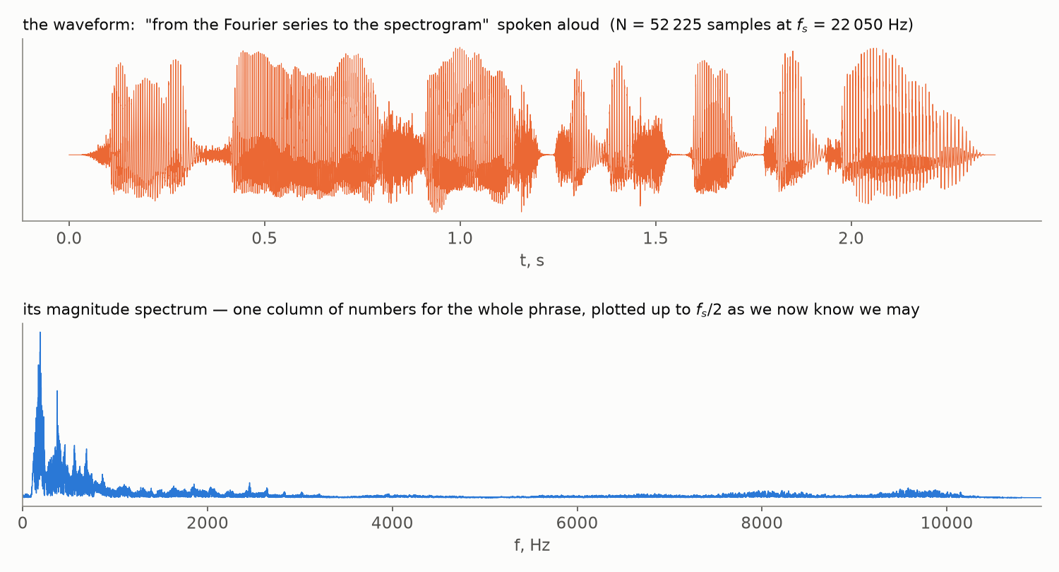
Notice the asymmetry in what the two pictures know. In the waveform you can practically count the words — bursts of energy separated by silences — but no frequencies are visible. The spectrum knows all the frequencies: the tall peaks on the left are the voice and its harmonics. But it is one column of numbers for the whole phrase — every phoneme’s frequencies stacked into the same bins, and when is gone entirely. A chord is a fine thing to summarize with one spectrum; a sentence is not: “which frequencies appear” is not the same as “which frequencies appear when”. In Part 3 we make the Fourier view local — slide a window along the recording, pay the resolution bill we just learned about at every stop, and stack the results into the picture this series is named after: the spectrogram.

Every computation of this part can be rerun and poked at: a ready-made notebook lives in this blog’s repository and opens in Colab in one click. It also covers the corner cases the post glossed over: the sine that vanishes at exactly the Nyquist frequency, what happens to the Nyquist bin when $N$ is odd, and the factor-of-2 bookkeeping of one-sided amplitude spectra (the same machinery scipy applies inside its one-sided routines).

Appendix: the probes are a basis

Back in What does X[k] measure?, the green model hit every sample dead on — and that was promised to be no accident. This interlude pays the debt — a stretch of honest linear algebra, ending with a reunion with an old classic.

First, write the model down. As a function of continuous time, the $k$-th probe is $e^{2 \pi i \frac{k}{NT} t}$ — the $k$-th grid frequency — so the weighted probe sum is

$$ \tilde{x}(t) = \frac{1}{N} \sum_{k=0}^{N-1} X[k]\, e^{2 \pi i \frac{k}{NT} t}. $$

Now put a sample instant $t = nT$ into it. The $T$ cancels in the exponent, and

$$ \tilde{x}(nT) = \frac{1}{N} \sum_{k=0}^{N-1} X[k]\, e^{2 \pi i \frac{k n}{N}} = x[n] $$

— the right-hand side is literally the inverse DFT formula from Part 1, and its output is the original samples. So at the grid instants the model has no freedom at all: it is contractually obliged to return $x[n]$.

That pushes the question one step deeper: why does the inverse formula reproduce the samples exactly? To see it, switch to vector language — and start slow. The inverse DFT is one equation per sample — write them all out, one under another:

$$ \begin{aligned} x[0] &= \tfrac{X[0]}{N}\, w_0[0] + \tfrac{X[1]}{N}\, w_1[0] + \dots + \tfrac{X[N-1]}{N}\, w_{N-1}[0] \\ x[1] &= \tfrac{X[0]}{N}\, w_0[1] + \tfrac{X[1]}{N}\, w_1[1] + \dots + \tfrac{X[N-1]}{N}\, w_{N-1}[1] \\ &\;\;\vdots \\ x[N-1] &= \tfrac{X[0]}{N}\, w_0[N-1] + \dots + \tfrac{X[N-1]}{N}\, w_{N-1}[N-1]. \end{aligned} $$

Now read this system by columns instead of rows. Every column carries one and the same scalar $\tfrac{X[k]}{N}$ — and the stack of numbers it multiplies, $w_k[0], w_k[1], \dots, w_k[N-1]$, is the $k$-th probe written out top to bottom. So the $N$ equations are really one equation between columns:

$$ \begin{pmatrix} x[0] \\ x[1] \\ \vdots \\ x[N-1] \end{pmatrix} = \frac{X[0]}{N} \begin{pmatrix} w_0[0] \\ w_0[1] \\ \vdots \\ w_0[N-1] \end{pmatrix} + \dots + \frac{X[N-1]}{N} \begin{pmatrix} w_{N-1}[0] \\ w_{N-1}[1] \\ \vdots \\ w_{N-1}[N-1] \end{pmatrix}. $$

Name the columns — $\mathbf{x}$ on the left, $\mathbf{w}_k$ for the $k$-th one on the right — and the whole system collapses into one line, with the forward transform alongside it. The second formula is nothing new: it is the inner-product form of the DFT from the very first section, now wearing vector notation:

$$ \mathbf{x} = \sum_{k=0}^{N-1} \frac{X[k]}{N}\, \mathbf{w}_k, \qquad X[k] = \langle \mathbf{x}, \mathbf{w}_k \rangle $$

So the claim to be proved now reads: measure the resemblances $X[k] = \langle \mathbf{x}, \mathbf{w}_k \rangle$, use them as weights — and the weighted probes reassemble $\mathbf{x}$ itself. One property of the probes does all the work here: as vectors, they are orthogonal to one another. Compute their inner product:

$$ \langle w_j, w_k \rangle = \sum_{n=0}^{N-1} e^{2 \pi i \frac{(j - k) n}{N}}. $$

For $j = k$ every term is $1$ and the sum is $N$. For two different probes it is a geometric series with ratio $q = e^{2 \pi i (j-k)/N}$ — a ratio that is not $1$ itself, yet satisfies $q^N = 1$ — so the sum, $\frac{q^N - 1}{q - 1}$, is exactly zero.

That settles everything. Orthogonal vectors are linearly independent, so the $N$ probes form a genuine basis of the $N$-dimensional space of sample lists — the word we have been using all along, now earned — and every $\mathbf{x}$ is a weighted sum of probes in exactly one way. And for an orthogonal basis, the weights are given by the textbook formula: the inner product with the basis vector, divided by that vector’s squared length. That is precisely our pair of formulas — with squared length $\langle \mathbf{w}_k, \mathbf{w}_k \rangle = N$, which is where the $\frac{1}{N}$ of the inverse DFT has been hiding all along. (Part 1’s convention inset told you where that factor is put; this is why it exists. And one step further, for the matrix-minded: stack the probes as the columns of an $N \times N$ matrix $W$; orthogonality reads $W^{*} W = N I$, so $W / \sqrt{N}$ is unitary — the DFT is, up to scale, a rotation of $\mathbb{C}^N$.)

One more name for the same matrix

Look at the entries of $W$ once more: $(W)_{nk} = w_k[n] = \omega^{nk}$ with $\omega = e^{2 \pi i / N}$, so the $n$-th row is $1, \omega^n, \omega^{2n}, \dots$ — the successive powers of a single number. A matrix whose rows are geometric progressions of their own “nodes”, $V_{jk} = z_j^{\,k}$, has a classical name: the Vandermonde matrix. Written out in full, with one node per row:

$$ V = \begin{pmatrix} 1 & z_0 & z_0^2 & \cdots & z_0^{N-1} \\ 1 & z_1 & z_1^2 & \cdots & z_1^{N-1} \\ \vdots & \vdots & \vdots & & \vdots \\ 1 & z_{N-1} & z_{N-1}^2 & \cdots & z_{N-1}^{N-1} \end{pmatrix}. $$

It is the matrix of polynomial interpolation — solving $V \mathbf{c} = \mathbf{y}$ means finding a polynomial with coefficients $c_k$ that passes through the points $(z_j, y_j)$ — and its famous determinant,

$$ \det V = \prod_{0 \,\le\, i \,\lt\, j \,\le\, N-1} (z_j - z_i), $$

says it is invertible exactly when all the nodes are distinct.

The DFT matrix, then, is the Vandermonde matrix with its nodes placed at the $N$-th roots of unity, $z_j = \omega^j$ — watch the rows fill in with powers of $\omega$:

$$ W = \begin{pmatrix} 1 & 1 & 1 & \cdots & 1 \\ 1 & \omega & \omega^2 & \cdots & \omega^{N-1} \\ 1 & \omega^2 & \omega^4 & \cdots & \omega^{2(N-1)} \\ \vdots & \vdots & \vdots & & \vdots \\ 1 & \omega^{N-1} & \omega^{2(N-1)} & \cdots & \omega^{(N-1)^2} \end{pmatrix}. $$

Nodes as distinct, and as symmetric, as $N$ points can be — and that special placement is what upgrades “invertible” to “unitary up to scale”. Two consequences are worth savoring.

First, our sample-hitting model turns out to be a polynomial interpolation problem, posed the most natural way: find the polynomial of degree $N-1$,

$$ q(z) = c_0 + c_1 z + \dots + c_{N-1} z^{N-1}, $$

whose values at the $N$ roots of unity are exactly our samples — one node per sample:

$$ q(\omega^n) = \sum_{k=0}^{N-1} c_k\, \omega^{k n} = x[n], \qquad n = 0, \dots, N-1. $$

Stare at this system of $N$ conditions: the matrix multiplying the unknown coefficients has entries $\omega^{nk}$ — it is exactly our $W$. Finding the polynomial through the samples means solving $W \mathbf{c} = \mathbf{x}$ — written out in full:

$$ \underbrace{\begin{pmatrix} 1 & 1 & \cdots & 1 \\ 1 & \omega & \cdots & \omega^{N-1} \\ \vdots & \vdots & & \vdots \\ 1 & \omega^{N-1} & \cdots & \omega^{(N-1)^2} \end{pmatrix}}_{W} \underbrace{\begin{pmatrix} c_0 \\ c_1 \\ \vdots \\ c_{N-1} \end{pmatrix}}_{\mathbf{c}} = \underbrace{\begin{pmatrix} x[0] \\ x[1] \\ \vdots \\ x[N-1] \end{pmatrix}}_{\mathbf{x}}. $$

And this system we can simply solve, because the inverse matrix costs nothing: a few paragraphs ago orthogonality gave us $W^{*} W = N I$, that is,

$$ W^{-1} = \frac{1}{N} W^{*}, \qquad\text{so}\qquad \mathbf{c} = \frac{1}{N} W^{*} \mathbf{x}. $$

Now look at what the product $W^{*} \mathbf{x}$ computes, row by row. Written out, the conjugate transpose is simply $W$ with the sign of every power flipped — conjugation negates the exponents, and transposition changes nothing because $W$ is symmetric:

$$ W^{*} = \begin{pmatrix} 1 & 1 & 1 & \cdots & 1 \\ 1 & \omega^{-1} & \omega^{-2} & \cdots & \omega^{-(N-1)} \\ 1 & \omega^{-2} & \omega^{-4} & \cdots & \omega^{-2(N-1)} \\ \vdots & \vdots & \vdots & & \vdots \\ 1 & \omega^{-(N-1)} & \omega^{-2(N-1)} & \cdots & \omega^{-(N-1)^2} \end{pmatrix}. $$

The $k$-th row holds the conjugated probe $\overline{w_k[n]} = \omega^{-k n}$, so the $k$-th entry of $W^{*} \mathbf{x}$ is $\sum_n x[n]\, \omega^{-k n}$ — the forward DFT, term for term. The solution of the interpolation system turns out to be our old coefficients:

$$ c_k = \frac{X[k]}{N}. $$

To interpolate through the samples, run a forward DFT — that is the entire algorithm. (Interpolation normally costs solving a linear system; this particular system’s matrix inverts by mere conjugation, because its columns are orthogonal.)

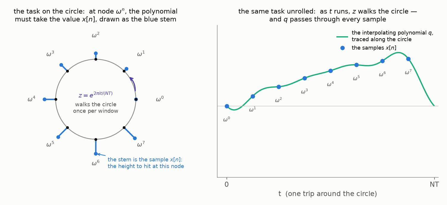
And the interpolating polynomial is an old friend. Substitute $z = e^{2 \pi i t / (NT)}$: as $t$ runs through the window, $z$ walks once around the unit circle, visiting the node $\omega^n$ exactly at the sample instant $t = nT$. Under this substitution — with the solution $c_k = X[k]/N$ plugged in on the second line —

$$ \begin{aligned} q\!\left( e^{2 \pi i t/(NT)} \right) &= \sum_{k=0}^{N-1} c_k\, e^{2 \pi i \frac{k}{NT} t} \\ &= \frac{1}{N} \sum_{k=0}^{N-1} X[k]\, e^{2 \pi i \frac{k}{NT} t} = \tilde{x}(t) \end{aligned} $$

— $q$ turns into $\tilde{x}(t)$, the green model from the pictures. The curve that hit every sample was this interpolating polynomial all along, traced along the circle:

A fine-print footnote: why the drawn curve is real (it leans on the mirror symmetry)

Traced literally with the frequencies $0, \dots, N-1$, the curve $q(e^{2 \pi i t/(NT)})$ is complex-valued between the samples. The drawn curve lets the mirror twins act as a conjugate pair instead: for $0 \lt k \lt N/2$ the coefficients $X[k]$ and $X[N-k] = \overline{X[k]}$ keep their full values, but the twin plays its negative frequency $k - N$ rather than $N - k$ — and the pair’s two terms, now complex conjugates of each other, sum to the real quantity $2 \operatorname{Re}\!\left( X[k]\, e^{2 \pi i k t/(NT)} \right)$. No averaging happens there; the only coefficient literally split in half is the lone Nyquist one when $N$ is even — half of $X[N/2]$ goes to $+f_s/2$, half to $-f_s/2$, and the halves sum to a real cosine. At the sample instants every one of these choices is indistinguishable, because $e^{2 \pi i (k-N) n/N} = e^{2 \pi i k n/N}$ — the periodicity $c_{k+N} = c_k$ yet again.

Second, this coefficients-to-values dictionary, cheap in both directions, is exactly how the FFT multiplies polynomials fast — convert both factors to their values at the roots of unity, multiply the values pointwise, convert the product back to coefficients — the trick at the heart of big-integer arithmetic.