From the Fourier Series to the Spectrogram, Part 1: From Sound to the DFT

Open any tutorial on speech processing and you will meet the spectrogram in the first five minutes — usually with a hand-wave: “we apply the Fourier transform in sliding windows”. Open a math textbook, and you will find the Fourier series in its full rigor — with no hint of why an ML engineer should care. The road between these two points is almost never walked end to end: every explanation starts somewhere in the middle. This series of three posts walks the whole road: from air pressure and a guitar string, through sampling and quantization, through the Fourier series and the DFT, to the spectrogram — the picture that speech models actually consume. In this first part we build the core machinery: we follow the sound wave into the computer and end with the DFT derived — honestly, delta functions and all — from the Fourier series itself.

Along the way we will meet several different creatures that all answer to the name “Fourier”: the Fourier series, the Fourier transform, its discrete-time cousin, and the discrete Fourier transform. They form a tidy 2×2 family — and untangling their family relationships is a story of its own, which gets a separate post (and more): for now, one picture as a teaser.

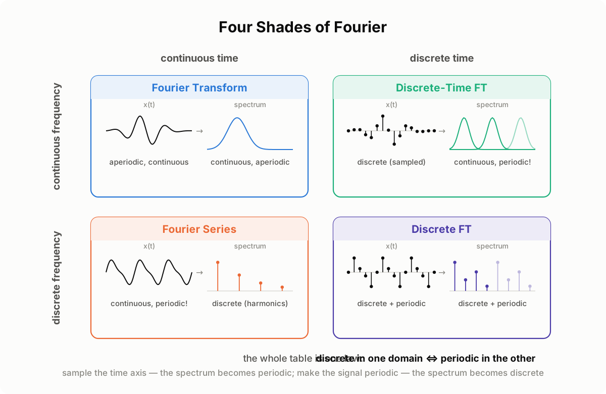
(a teaser of a separate post to come — in this series we walk the bottom row: from the Fourier series to the discrete Fourier transform)

What is sound

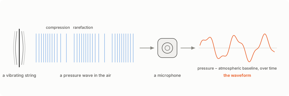
The air around us is filled with molecules. Pull a guitar string — it creates a vibration that travels through them as alternating zones of compression and rarefaction: a pressure wave. A microphone senses exactly this: variations of pressure relative to the atmospheric baseline. Plot that pressure against time — and you get the most honest picture of sound there is: the waveform.

💡 Sound is a mechanical wave — it needs a medium. In the vacuum of space there is nothing to compress, which is why we can see the Sun but cannot hear it.

Analog → digital

The microphone’s output is an analog signal — and the word is more literal than it sounds: the voltage on the microphone’s wire is an analogue of the air pressure, one physical quantity tracing the shape of another. Nothing has been measured yet; the signal has merely changed its carrier — from pressure to voltage — and is still continuous in time and in value.

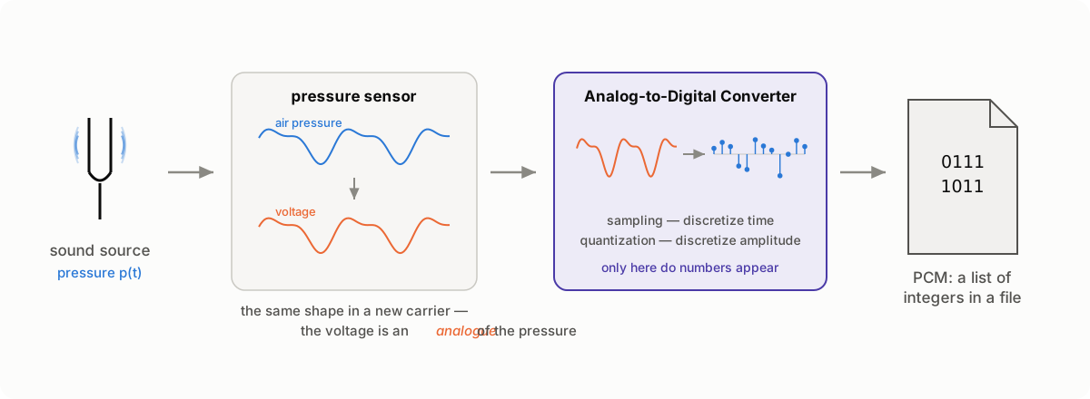
A computer, however, needs numbers, and the Analog-to-Digital Converter (ADC) produces them by discretizing along both axes:

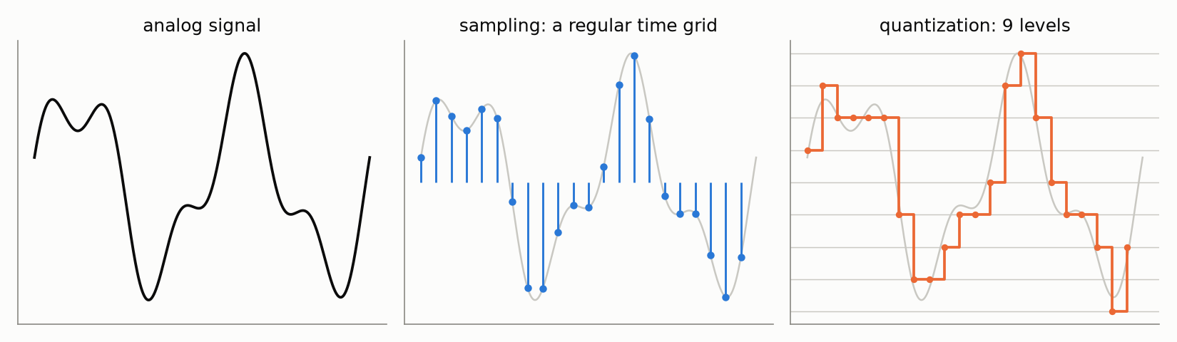
• sampling — measure the signal at regular moments, $f_s$ times per second (time discretization);
• quantization — round each measurement to the nearest level of a fixed grid (amplitude discretization).

The result — a sequence of integers at a fixed rate — is Pulse-Code Modulation (PCM), the format inside every .wav file. Two numbers fully describe the grid: the sampling rate (e.g. 44.1 kHz) and the bit depth (e.g. 16 bits).

Why the waveform is not enough

The waveform is honest but unhelpful. One second of CD-quality audio is 44,100 numbers — and no individual number tells you anything about what you hear. Is this a male or a female voice? Which note is the guitar playing? Is there a hum from the power line polluting the recording? Staring at pressure values will not answer any of these questions.

Fourier’s idea flips the axis. A complex signal can be decomposed into a sum of simple oscillations — the way a chord can be decomposed into individual notes. Instead of asking “what is the pressure at each moment of time?”, we ask “how much of each frequency does this signal contain?” The answer lives on the frequency axis rather than the time axis, and it is called the spectrum.

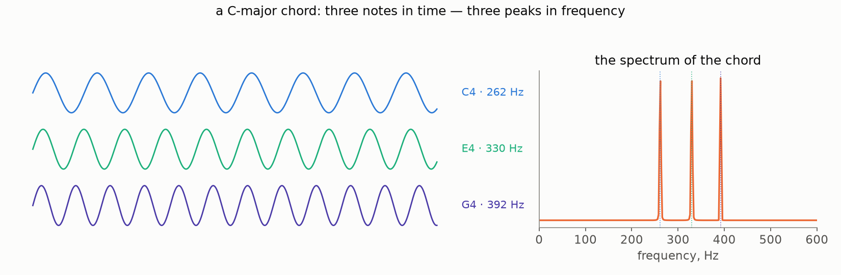
If decomposing sound into frequencies feels like an arbitrary idea, think of a piano. Pressing a key produces an oscillation at a known frequency — the keyboard is literally a frequency axis, laid out left to right. Playing music is easy in this direction: choose which keys to press, how hard, and when — frequencies in, melody out. Fourier analysis asks for the reverse: given only the recorded sound, can we recover which keys were pressed and how hard? Most of this post is the machinery that turns this “can we?” into “here is how”.

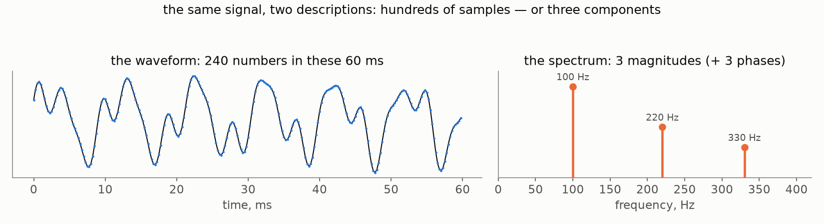
Two things make this representation valuable in practice. First, it is compact: a long sequence of time samples collapses into a handful of meaningful frequency components. The wiggly curve below takes hundreds of numbers to store — and just three frequency components to describe:

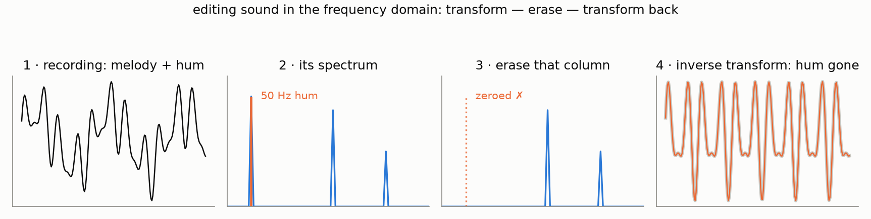
Second, it is actionable: frequencies can be inspected and edited. Say a recording picked up the 50 Hz hum of the power line. In the time domain the hum is smeared over every sample and there is nothing to grab; in the frequency domain it is one column. Transform, erase that column, transform back — the melody survives untouched, the hum is gone:

The Fourier series

Let us make the “sum of simple oscillations” idea precise. We start with the version that history started with, too: a periodic function.

Any periodic function $x(t)$ with period $P$ that is absolutely integrable over $\left[-\frac{P}{2}, \frac{P}{2}\right]$ can be represented as a Fourier series:

$$ x(t) = a_0 + \sum_{n = 1}^\infty \left( a_n \cos\!\left( 2 \pi \frac{n}{P} t \right) + b_n \sin\!\left( 2 \pi \frac{n}{P} t \right) \right) $$

with the coefficients

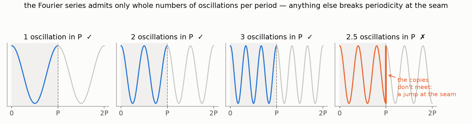
$$ \begin{gathered} a_0 = \frac{1}{P} \int_{-P/2}^{P/2} x(t)\, dt, \\ a_n = \frac{2}{P} \int_{-P/2}^{P/2} x(t) \cos\!\left(2 \pi \frac{n}{P} t \right) dt, \qquad b_n = \frac{2}{P} \int_{-P/2}^{P/2} x(t) \sin\!\left(2 \pi \frac{n}{P} t \right) dt. \end{gathered} $$

The building blocks are sines and cosines whose frequencies are integer multiples of $\frac{1}{P}$ — the harmonics of the base frequency. Nothing else is allowed: only oscillations that fit a whole number of times into the period. This restriction is easy to read past, and much of what follows grows out of it — so let us stare at it once, properly. A periodic function repeats: whatever happens on $[0, P]$ must glue seamlessly to its own copy on $[P, 2P]$. A harmonic with a whole number of oscillations arrives at the seam exactly where it started, so the copies join smoothly. An oscillation with a fractional count arrives somewhere else — and the glued copies tear:

A pair $(a_n, b_n)$ at the same frequency is really one oscillation in disguise. Using the cosine-of-difference formula, the pair collapses into a single cosine with an amplitude and a shift:

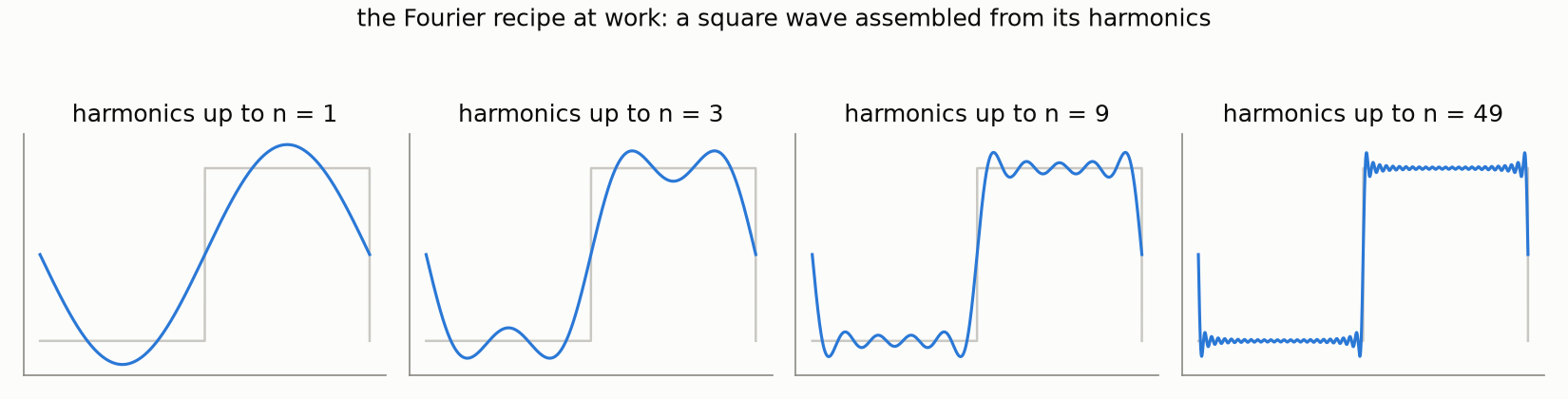
$$ \begin{gathered} x(t) = a_0 + \sum_{n = 1}^\infty A_n \cos\!\left( 2 \pi \frac{n}{P} t - \phi_n\right), \\ A_n = \sqrt{a_n^2 + b_n^2}, \qquad \phi_n = \operatorname{atan2}(b_n, a_n). \end{gathered} $$

Here $A_n$ is the magnitude of the $n$-th harmonic, $\frac{n}{P}$ its frequency, and $\phi_n$ its phase. This form is the one to keep in mind: a periodic signal is a recipe — this much of this frequency, shifted by this much.

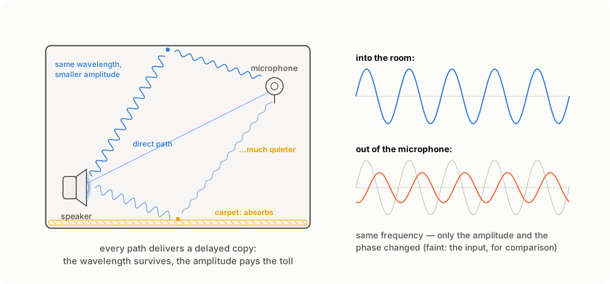
💡 Why sinusoids, of all things? Mathematics knows plenty of ways to decompose a function — why not, say, a Taylor series, with polynomials as the building blocks? Several reasons stack on top of each other. First, the shape of the data: sound is locally quasi-periodic — a guitar note, a vowel — and periodic building blocks describe such signals with a handful of coefficients, while a polynomial cannot even be periodic (it must run off to infinity) and needs ever more terms for every extra period. Second, and deeper: the physical world plays along. Put a speaker in one corner of a room, play a pure 440 Hz tone through it, and record with a microphone in the opposite corner. The walls reflect the sound, echoes pile on top of each other — yet the recording is still a 440 Hz tone: louder or quieter, shifted in time, but at the same frequency. The reason is one line of trigonometry: echoes are delayed, scaled copies, and a sum of sinusoids of one frequency — whatever their amplitudes and shifts — is again a sinusoid of that frequency.

(Can a room be an anti-carpet and make a frequency louder? It cannot add energy — but it can concentrate it: when the copies arrive in phase, they add up constructively. That is resonance, and it is exactly why your voice blossoms in a tiled bathroom — at the room’s resonant frequencies, the echoes conspire in your favor.)

The same holds for a vibrating string, a microphone membrane, an electronic filter: none of them can invent new frequencies. (A distortion pedal can — precisely because it is not linear; that is what its “dirty” sound is made of.) That is why sound is built out of sinusoids in the first place, and the quasi-periodicity of the previous argument is not a lucky accident but physics. (Why this happens — and why it earns sinusoids the grand title of eigenfunctions of linear time-invariant systems — is a story of its own; for a very accessible account, see chapter 5 of The Scientist and Engineer’s Guide to DSP.) Third, stability. To compare fairly, fix the reference point — the moment you press “record” — and delay the signal past it by $\tau$. The Fourier description barely notices: delaying the signal turns each harmonic $A_n \cos(2\pi \frac{n}{P} t - \phi_n)$ into $A_n \cos(2\pi \frac{n}{P} (t - \tau) - \phi_n)$ — which is the same cosine with the same magnitude $A_n$, only its phase nudged to $\phi_n + 2\pi \frac{n}{P} \tau$. The Taylor description — the derivatives at the reference point — has no such luck: every new coefficient becomes a mixture of all the old higher-order ones. The cleanest example: $\sin t$ and $\cos t$ are one signal shifted by a quarter period, yet one has only odd-degree terms and the other only even-degree ones. A note sounds the same whenever you play it, and the magnitude spectrum agrees; the Taylor coefficients do not. (It is the room argument again, in disguise: a time shift leaves every sinusoid being itself, just rotated — while it smears each monomial $t^k$ across all the degrees below it.)

The exponential form

One more rewrite, and the notation becomes so compact that every later formula in this series will use it. Euler’s formula,

$$ e^{i t} = \cos t + i \sin t \quad\Longleftrightarrow\quad \cos t = \tfrac{1}{2} \left(e^{it} + e^{-it} \right), $$

lets us split every cosine into two complex exponentials — one rotating “forward” and one “backward”:

$$ \cos\!\left( 2 \pi \tfrac{n}{P} t - \phi_n \right) = \tfrac{1}{2} e^{-i \phi_n} e^{2 \pi i \frac{n}{P} t} + \tfrac{1}{2} e^{i \phi_n} e^{-2 \pi i \frac{n}{P} t}. $$

Absorbing the magnitudes and phases into complex coefficients, the whole series collapses into a single sum:

$$ x(t) = \sum_{n = -\infty}^\infty c_n e^{2 \pi i \frac{n}{P} t}, \qquad c_n = \frac{1}{P} \int_{-P/2}^{P/2} x(t)\, e^{-2 \pi i \frac{n}{P} t}\, dt. $$

The set of coefficients $\{c_n\}$ is called the spectrum of the signal — the same word we met informally above, now with an exact meaning. Each $c_n$ is one complex number that stores both the magnitude and the phase of the $n$-th harmonic: $|c_n| = A_n / 2$ and $\arg c_n = -\phi_n$ for $n \ge 1$.

💡 Wait, negative frequencies? The sum now runs over all integers $n$, including negative ones — that is the price of the compact notation: each real oscillation split into a forward- and a backward-rotating exponential. For a real-valued signal the two halves are not independent: $c_{-n} = \overline{c_n}$, so the negative-frequency half of the spectrum is a mirror image carrying no new information. Remember this — the same symmetry will resurface in the DFT and explain why half of its coefficients can be thrown away.

From the series to the DFT

This is the part most explanations skip. Textbooks stop at the Fourier series for nice continuous functions; engineering tutorials start from the DFT formula, presented as an axiom. But the road between them is short, honest, and worth walking — and it starts where honesty demands: by asking what a sampled signal even is as a mathematical object.

An honest model of a discrete signal

Remember the Analog-to-Digital Converter from the digitization section, back before all the mathematics? It is about to become the protagonist again:

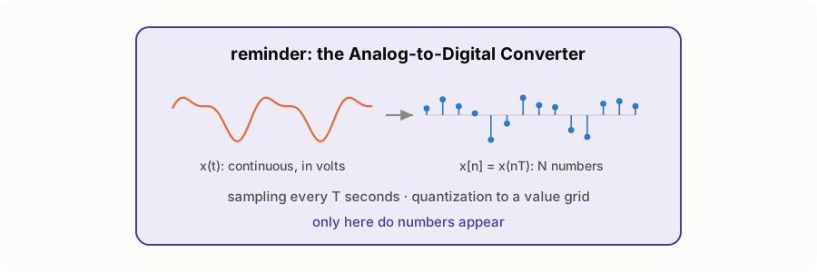
This is what it left us with: $N$ numbers $x(0), x(T), \dots, x\big((N-1)T\big)$, measured every $T$ seconds. Can we recover a spectrum from these points? A spectrum means Fourier coefficients, and coefficients are integrals — so before computing anything, we owe the integral a well-definedness check. For a bounded function, the Riemann integral exists precisely when the function is continuous almost everywhere: its discontinuities must form a set of measure zero — this is Lebesgue’s integrability criterion.

Our samples are not yet a function of continuous time, so let us complete them in the most straightforward way imaginable: keep the measured values at the grid points, put zero everywhere else,

$$ \tilde{x}(t) = \begin{cases} x(nT), & t = nT, \quad n = 0, \dots, N-1, \\ 0, & t \in [0, NT], \; t \neq nT. \end{cases} $$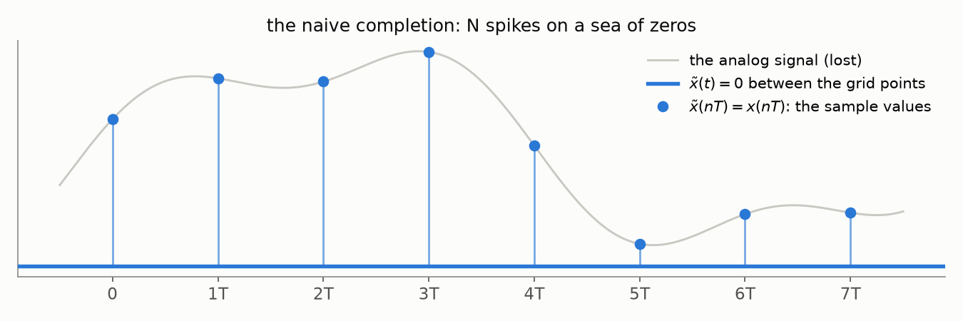

Does $\tilde{x}$ pass the check? It is bounded; and it is discontinuous only at the grid points — finitely many on one period, and still just countably many after the periodic extension that the series insists on. A countable set has measure zero — continuous almost everywhere, check. The coefficients are well-defined, and we may integrate with a clear conscience:

$$ c_k = \frac{1}{P} \int_{0}^{P} \tilde{x}(t)\, e^{-2 \pi i \frac{k}{P} t}\, dt \equiv 0 \quad \text{for every } k. $$

Every single coefficient is zero — our signal has vanished from the mathematics. To see why, watch the Riemann sums converge: each spike gets trapped in a rectangle of finite height and ever-shrinking width, so its contribution — height times width — dies together with the mesh. Countably many spikes stand against a continuum of zeros, and the zeros win:

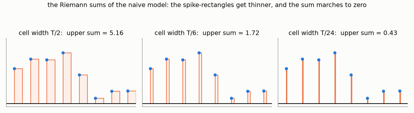
The integral honestly reports that $\tilde{x}$ is almost everywhere indistinguishable from the zero function. The verdict is not against Fourier; it is against our model: “a value at a point and zero elsewhere” is the wrong mathematical object for a sample.

So what is a sample, really? Think about how the measurement is actually made. No instrument reads a value at an instant — a measurement takes some time $\tau$: around every grid point $t = nT$ the device opens its gate, and for $\tau$ seconds the signal pours in:

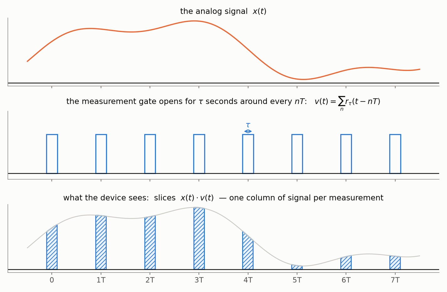
What single number should the device report for its window? It saw not one value but a continuum of them — everything the signal did between $nT - \tau/2$ and $nT + \tau/2$. The natural answer is the average. And what is the average of a continuum of values? For a handful of numbers the average is “add them up, divide by how many”; for a continuum, the sum becomes an integral and the count becomes the length of the window:

$$ \hat{x}(nT) = \frac{1}{\tau} \int_{nT - \tau/2}^{nT + \tau/2} x(t)\, dt. $$

It is useful to rewrite this average as an integral against a kernel. Let $r_\tau(t)$ be the rectangular pulse of width $\tau$ and unit height centered at zero:

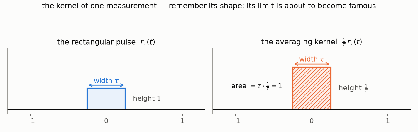
With the scaled pulse as the kernel, the average becomes

$$ \hat{x}(nT) = \int_{-\infty}^{\infty} x(t)\, \tfrac{1}{\tau} r_\tau(t - nT)\, dt. $$

The kernel $\frac{1}{\tau} r_\tau$ cuts a column of width $\tau$ out from under the graph of $x$ and reports its area, divided by the width — the average height of the graph inside the window. Remember this shape: it is about to have a famous limit. For finite $\tau$ this is an estimate with an error: the signal keeps changing inside the window.

Now improve the instrument. As $\tau$ shrinks, the kernel becomes a rectangle ever narrower and ever taller — width $\tau$, height $\frac{1}{\tau}$, area always exactly $1$ — and the estimate sharpens:

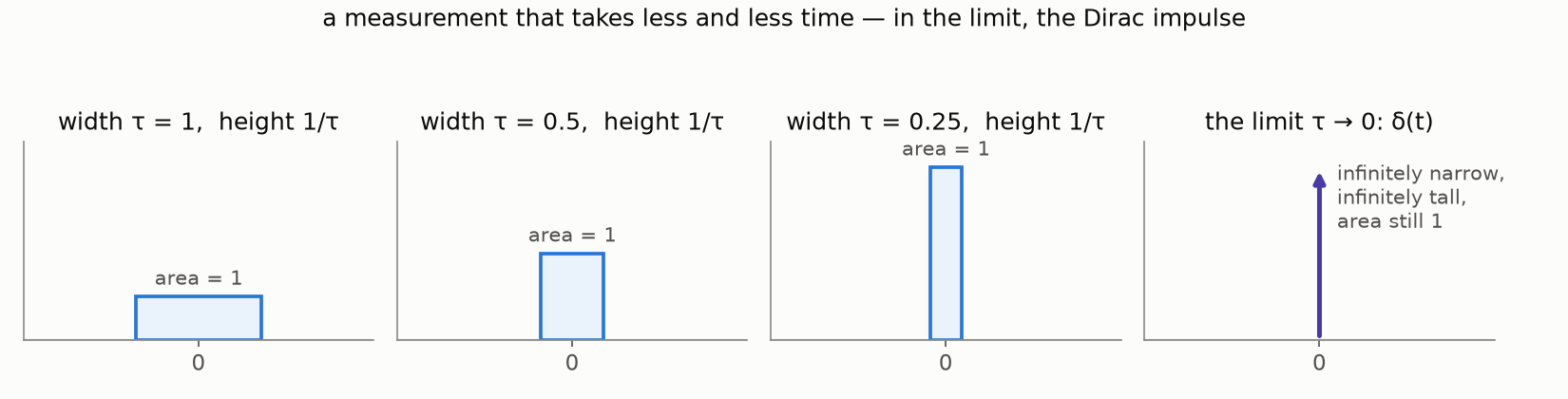
The limit of this process,

$$ \delta(t) = \lim_{\tau \to 0} \tfrac{1}{\tau} r_\tau(t), $$

is the Dirac impulse: an “infinitely narrow, infinitely tall” spike of unit area. It is not a function in the classical sense — it is defined by what it does inside an integral, namely the sifting property, the $\tau \to 0$ limit of our averaging:

$$ \int_{-\infty}^{\infty} x(t)\, \delta(t - t_0)\, dt = x(t_0) $$

— and any integration limits that enclose $t_0$ work just as well, since the spike carries all of its area at the single point $t_0$.

Proof of the sifting property (a physicist's proof: we swap limits and integrals without asking permission)

Step 0: a notation. For two real square-integrable signals (the space $L^2$ — where the Cauchy–Schwarz inequality guarantees the integral below is finite), their scalar (inner) product is

$$ \langle f(t), g(t) \rangle = \int_{-\infty}^{\infty} f(t)\, g(t)\, dt $$

— the continuous cousin of the dot product of vectors: multiply the two signals pointwise, then add everything up (with the sum, as usual by now, becoming an integral; complex signals conjugate the second factor). In this notation, the sifting property reads $\langle x(t), \delta(t - t_0) \rangle = x(t_0)$.

Step 1: the spike at zero. Substitute the definition of $\delta$ as the limit of our rectangles and move the limit outside the integral:

$$ \begin{aligned} \langle x(t), \delta(t) \rangle &= \int_{-\infty}^{\infty} x(t)\, \delta(t)\, dt = \int_{-\infty}^{\infty} x(t) \lim_{\tau \to 0} \tfrac{1}{\tau} r_\tau(t)\, dt \\ &= \lim_{\tau \to 0} \int_{-\infty}^{\infty} x(t)\, \tfrac{1}{\tau} r_\tau(t)\, dt. \end{aligned} $$

Step 2: the integral as a Riemann sum. Note what Step 1 bought us: a Riemann sum needs the values of the integrand at the grid points, and the original integrand contained $\delta(t)$ — which has no value at zero to sample. After the trade, for each fixed $\tau$ the integrand $x(t)\, \frac{1}{\tau} r_\tau(t)$ is an ordinary bounded function, and sampling it is legal. So write the integral as the limit of rectangle areas, choosing the mesh width to be the same $\tau$ as in the pulse (a shortcut of the genre: the mesh refinement and the pulse shrinkage merge into a single limit):

$$ \int_{-\infty}^{\infty} f(t)\, dt = \lim_{\tau \to 0} \sum_{n=-\infty}^{\infty} f(n\tau)\, \tau. $$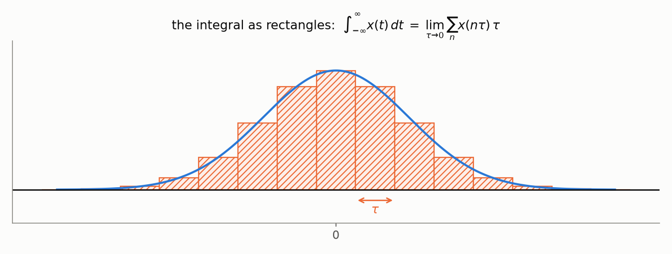

Applying this to our integrand, the $\tau$ of the mesh cancels the $\frac{1}{\tau}$ of the kernel:

$$ \begin{aligned} \langle x(t), \delta(t) \rangle &= \lim_{\tau \to 0} \sum_{n=-\infty}^{\infty} x(n\tau)\, \tfrac{1}{\tau} r_\tau(n\tau)\, \tau \\ &= \lim_{\tau \to 0} \sum_{n=-\infty}^{\infty} x(n\tau)\, r_\tau(n\tau). \end{aligned} $$

To be clear, this is where the genre’s quiet cheat actually lives. Honestly there are two independent limits — a mesh $h \to 0$ that defines the integral at each fixed $\tau$, and only then $\tau \to 0$ for the pulse. Setting $h = \tau$ walks a single diagonal path through a double limit, and diagonals are not automatically legal. Here the diagonal happens to be right: with the mesh equal to the pulse width, the sum quietly replaces the average of $x$ over the window by its value at the window’s midpoint, and the error of that replacement dies with $\tau$ by continuity — which is exactly what the Bonus section below proves properly.

Step 3: one term survives. The pulse $r_\tau$ is zero outside its window of width $\tau$ around zero — so of all the grid points $n\tau$, only $n = 0$ lands inside. The infinite sum collapses to a single term:

$$ \langle x(t), \delta(t) \rangle = \lim_{\tau \to 0} x(0) \underbrace{r_\tau(0)}_{=\,1} = x(0). $$

Step 4: the shifted spike. For $\delta(t - t_0)$, change variables $\xi = t - t_0$ (so $t = \xi + t_0$, $dt = d\xi$, and the infinite limits stay infinite):

$$ \int_{-\infty}^{\infty} x(t)\, \delta(t - t_0)\, dt = \int_{-\infty}^{\infty} x(\xi + t_0)\, \delta(\xi)\, d\xi = x(t_0) $$

by the case we just proved — the spike always reports the value of $x$ at the point where it stands. $\blacksquare$

Bonus: can the limit swap in Step 1 be saved by a theorem? A natural hope: perhaps uniform convergence, or Lebesgue’s dominated convergence, justifies moving the limit outside the integral? Here is the surprise — no theorem can, because the equality they would justify is false. The pointwise limit of $\frac{1}{\tau} r_\tau(t)$ is zero at every $t$ except the single point $t = 0$, where it blows up to $\infty$. Strictly speaking, “the integral of the limit” therefore does not even exist: the limit function is unbounded, and the proper Riemann integral is defined only for bounded functions — the very criterion we checked earlier. And if we repair the lone point (assign any finite value at $t = 0$, or integrate in the Lebesgue sense, where a single point has measure zero), the integral of a function that is zero almost everywhere is $0$. Either way — nonexistent or zero — the left-hand side is certainly not $x(0)$, and any theorem permitting the swap would be proving nonsense. Accordingly, every hypothesis fails on purpose. The convergence is not uniform — uniformity would demand $\sup_t \big| \frac{1}{\tau} r_\tau(t) \big| \to 0$, the whole graph fitting into an ever-thinner tube around zero, whereas our supremum is $\frac{1}{\tau}$ and blows up instead. And no integrable dominating function exists — at a fixed $t$, the largest value of $\frac{1}{\tau} r_\tau(t)$ over all $\tau$ is $\frac{1}{2|t|}$, and $\frac{1}{2|t|}$ is not integrable near zero.

The honest classical route runs in the opposite direction: swap the roles. Since “integrate the limit” is meaningless, we declare that the expression $\langle x(t), \delta(t) \rangle$ shall mean “the limit of the integrals”:

$$ \langle x(t), \delta(t) \rangle \;\overset{\text{def}}{=}\; \lim_{\tau \to 0} \int_{-\infty}^{\infty} x(t)\, \tfrac{1}{\tau} r_\tau(t)\, dt. $$

At each fixed $\tau$ everything inside is classical — a bounded integrand, an ordinary integral — and only after integrating do we let $\tau \to 0$. This limit we can compute directly. For a fixed $\tau$ there is no delta anywhere in sight:

$$ \int_{-\infty}^{\infty} x(t)\, \tfrac{1}{\tau} r_\tau(t)\, dt = \frac{1}{\tau} \int_{-\tau/2}^{\tau/2} x(t)\, dt $$

— the plain average of $x$ over the window. By the mean value theorem for integrals, for continuous $x$ this average equals $x(\xi_\tau)$ for some point $\xi_\tau$ inside the window; as $\tau \to 0$ the window collapses, $\xi_\tau \to 0$, and continuity gives $x(\xi_\tau) \to x(0)$. Fully rigorous — for continuous signals. Families like $\frac{1}{\tau} r_\tau$ are called approximate identities, or mollifiers: they are how analysis makes the delta respectable without ever letting it exist as a function.

A closing caveat in the same physicist’s spirit: the delta itself is famously not square-integrable, so $\langle x, \delta \rangle$ is not a true $L^2$ inner product — the angle brackets are a convenient notation for the pairing our formulas suggest. The bonus above makes our particular computation honest for continuous $x$; making the whole delta calculus systematic — for far rougher objects than continuous signals — is the job of distribution theory.

The perfect instrument, then, measures $x(nT)$ by integrating $x$ against $\delta(t - nT)$. Place one impulse at every grid point — the infinite train of shifted deltas is called the Dirac comb (the Russian DSP literature knows it as the lattice function):

$$ \text{Ш}_T(t) = \sum_{n=-\infty}^{\infty} \delta(t - nT), $$

and the honest model of a discrete signal is the analog signal multiplied by the comb (we follow the construction from ru.dsplib.org, archived):

$$ x_d(t) = x(t) \cdot \text{Ш}_T(t) = \sum_{n} x(t)\, \delta(t - nT). $$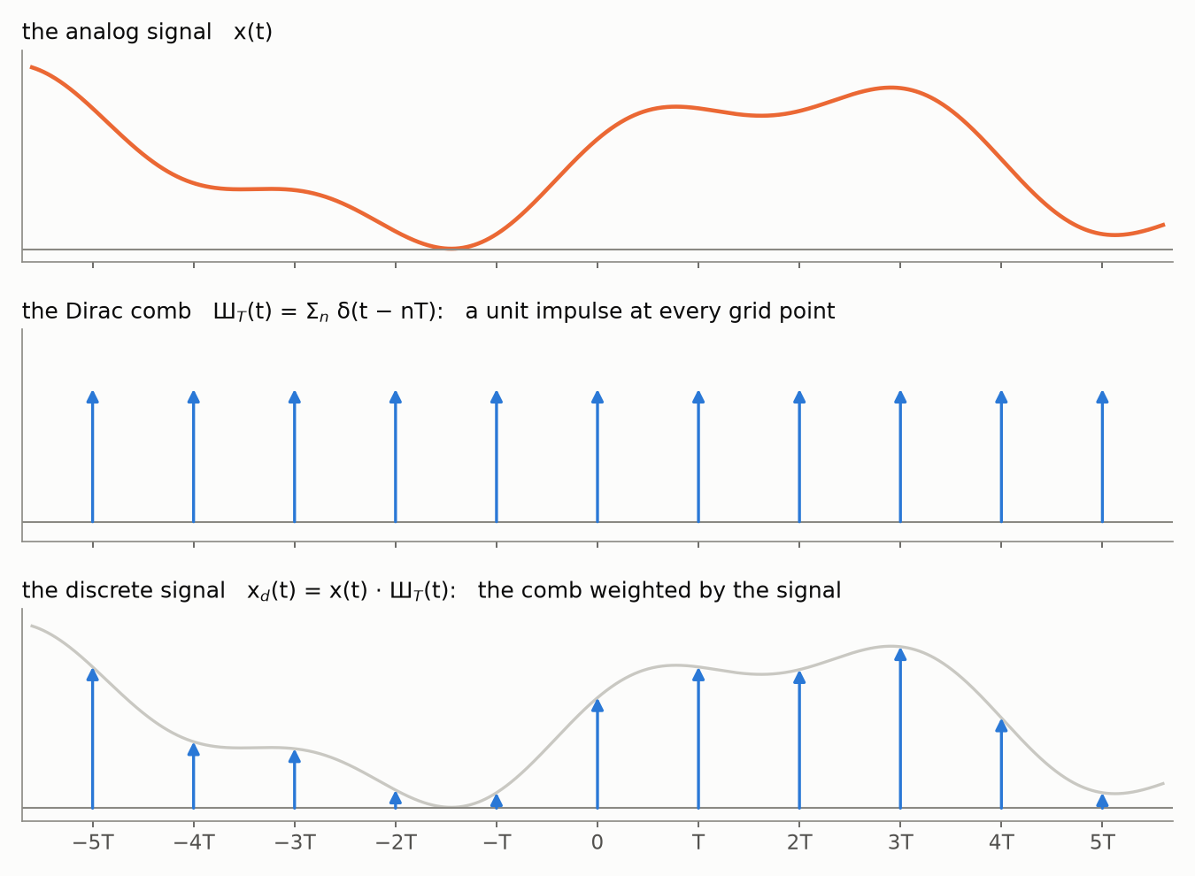

Note that nothing here is approximate anymore: the finite-$\tau$ estimate $\hat{x}$ with its error stayed behind in the limit. This is the exact mathematical model, the one the rest of the derivation stands on.

Did it fix the integration? Let us check — integrate $x_d$ in a small neighborhood of a sampling point $t_0 = kT$, taking limits $kT \pm \tau$ with $\tau \lt T$ so that exactly one tooth of the comb falls inside:

$$ \begin{aligned} \int_{kT - \tau}^{kT + \tau} x(t) \left( \sum_{n} \delta(t - nT) \right) dt &= \int_{kT - \tau}^{kT + \tau} x(t)\, \delta(t - kT)\, dt \\ &= x(kT), \end{aligned} $$

where the first equality holds because all the deltas except $n = k$ sit outside the integration limits. The integral no longer returns zero — it returns the sample. The sampling points survive integration, which is exactly what the naive model could not do.

💡 Yes, that symbol is a Cyrillic letter. The comb is traditionally denoted by Ш — “sha” — and Western literature adopted both the symbol and the name: the Shah function. It is quite possibly the only Cyrillic letter in standard mathematical notation, chosen for the obvious reason: the letter looks like the comb.

💡 A units check (a detail dsplib is careful about, and most sources skip): $\delta(t)$ has dimension $1/\text{time}$ — its area over time is the dimensionless $1$. So if $x(t)$ is in volts, the model $x_d(t)$ is in volts per second: it is a density, not a value — in the same sense as a probability density, whose pointwise values are not probabilities (they can even exceed $1$); only its integrals are. Here too the pointwise values of $x_d$ are useless — zero between the grid points, “infinite” on them — and the sample lives in the impulse’s area, not its height. The volts come back when you integrate — as we just saw. Keep this in mind whenever a stray $T$ or $\frac{1}{T}$ appears in sampling formulas — it is usually this density speaking.

Now bring in the series

Time to cash in. Remember where this whole detour started: we had $N$ samples out of the ADC and wanted their spectrum, but on the naive model the Fourier coefficient formula returned $c_k \equiv 0$ — the integrals looked straight through the isolated points. That is what sent us rebuilding the model. Now we hold $x_d$, whose integrals do see the samples — so this is attempt number two at the very same computation.

The Fourier series has one more requirement, though: a periodic function. Our recording is time-limited — so extend it, gluing copies of the $N$-sample stretch end to end. The smallest period that works is $P = NT$, the duration of the recording itself:

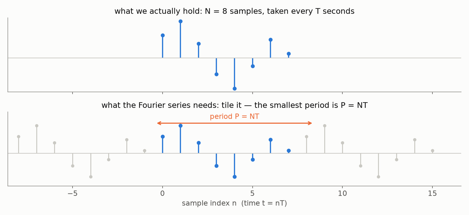
Feed the periodically extended comb into the Fourier coefficient formula. Over one period $[0, NT)$ exactly $N$ teeth of the comb fall inside, so under the integral sits a finite sum — and swapping a finite sum with an integral is plain linearity, no anxieties about interchanging limits this time. After the swap each summand is a sifting integral, and it evaluates the exponential at its grid point $t = nT$:

$$ \begin{aligned} c_k &= \frac{1}{NT} \int_{0}^{NT} x_d(t)\, e^{-2 \pi i \frac{k}{NT} t}\, dt \\ &= \frac{1}{NT} \sum_{n=0}^{N-1} \int_{0}^{NT} x(t)\, \delta(t - nT)\, e^{-2 \pi i \frac{k}{NT} t}\, dt \\ &= \frac{1}{NT} \sum_{n=0}^{N-1} x(nT)\, e^{-2 \pi i \frac{k}{NT} \cdot nT} = \frac{1}{NT} \sum_{n=0}^{N-1} x(nT)\, e^{-2 \pi i \frac{k n}{N}}. \end{aligned} $$

The dreaded integral has collapsed into a finite sum. And look at what happened in the exponent: the sampling period $T$ cancelled out. The basis functions no longer care about seconds — only about the two integers $k$ and $n$. The continuous world has quietly left the stage.

Only N distinct coefficients

The formula above is valid for any integer $k$ — but try shifting $k$ by $N$:

$$ e^{-2 \pi i \frac{(k+N) n}{N}} = e^{-2 \pi i \frac{k n}{N}} \underbrace{e^{-2 \pi i n}}_{=\,1} = e^{-2 \pi i \frac{k n}{N}}, $$

so $c_{k+N} = c_k$: the coefficients repeat with period $N$. Of the infinitely many harmonics the Fourier series offered us, only $N$ are genuinely distinct. $N$ numbers in, $N$ numbers out — the books balance.

And notice that both laws from the Four Shades table at the top of the post have just fired, each with its own culprit. Our spectrum is discrete — a list of coefficients $c_k$ rather than a function of a continuous frequency — because we periodized the signal: that is the Fourier series’ side of the bargain, baked in from the start. And the spectrum is periodic because the signal is sampled: look back at the computation — the whole proof of $c_{k+N} = c_k$ hangs on $e^{-2 \pi i n} = 1$, which is true only because $n$ is an integer, i.e. because the signal lives on a grid. Periodic in time ⇒ discrete in frequency; discrete in time ⇒ periodic in frequency. Not analogies — theorems, and we walked into both bottom-up.

The Discrete Fourier Transform

One last cosmetic step: new notation to mark the new attitude. The basis functions have forgotten about $T$, so let the signal forget it too — treat the input as a plain list of numbers and write

$$ x[n] \overset{\text{def}}{=} x(nT), $$

where the square brackets signal “the $n$-th entry of a list”, not “the value at a moment of time”. Drop the overall $\frac{1}{NT}$ factor as well (a convention we will revisit in a second) and call what remains $X[k]$ — the Discrete Fourier Transform:

$$ X[k] = \sum_{n=0}^{N-1} x[n]\, e^{-2 \pi i \frac{k n}{N}}, \qquad k = 0, 1, \dots, N-1, $$

and its inverse, which reassembles the samples from the spectrum:

$$ x[n] = \frac{1}{N} \sum_{k=0}^{N-1} X[k]\, e^{2 \pi i \frac{k n}{N}}, \qquad n = 0, 1, \dots, N-1. $$

💡 Where did the $\frac{1}{N}$ go? Between the forward and the inverse transform, a total factor of $\frac{1}{N}$ must appear somewhere — but the two formulas only constrain the product of their scale factors. The common engineering convention puts all of it into the inverse (as above), because the forward transform is computed far more often; a symmetric convention with $\frac{1}{\sqrt{N}}$ on both sides also exists and makes the transform unitary. Libraries differ — always check before comparing numbers.

The pair is an exact, lossless round trip: $N$ complex coefficients fully encode $N$ samples. And computing it is cheap: the naive sum costs $O(N^2)$ operations, but the Fast Fourier Transform computes exactly the same $X[k]$ in $O(N \log N)$ — the algorithmic miracle that makes everything downstream (including every spectrogram ever displayed) practical. This video is a beautiful walkthrough of the idea.

So here is what this part promised: an honest model of sampling, a periodic extension, and the Fourier series itself handed us the DFT — no axioms required. The machinery for “which piano keys were pressed?” is built.

In Part 2 we put the machinery to work and learn to read its output: what the $N$ complex numbers $X[k]$ actually say about the sound, which physical frequencies they correspond to, why half of them mirror the other half, and what limits the frequency resolution. In Part 3 the DFT starts sliding along the signal — windows, the short-time Fourier transform, and finally the spectrogram itself.