Four Shades of Fourier

Back in Part 1 of the spectrogram series we promised that several different creatures answer to the name “Fourier”, showed a 2×2 table as a teaser, and walked its bottom row — from the Fourier series to the discrete Fourier transform. (Throughout this post, “Part 1”, “Part 2” and “Part 3” refer to the parts of that series — this post itself is not a Part 4, just a close relative.) This post is the payoff of that teaser: we meet the remaining shades — the Fourier transform and its discrete-time cousin — and, more importantly, build every bridge between the four. None of the four is an axiom; each is another one pushed through a limit, a sampling, or a periodization.

Here is the whole map at once — the four shades in their corners, and the five bridges numbered in the order we will cross them:

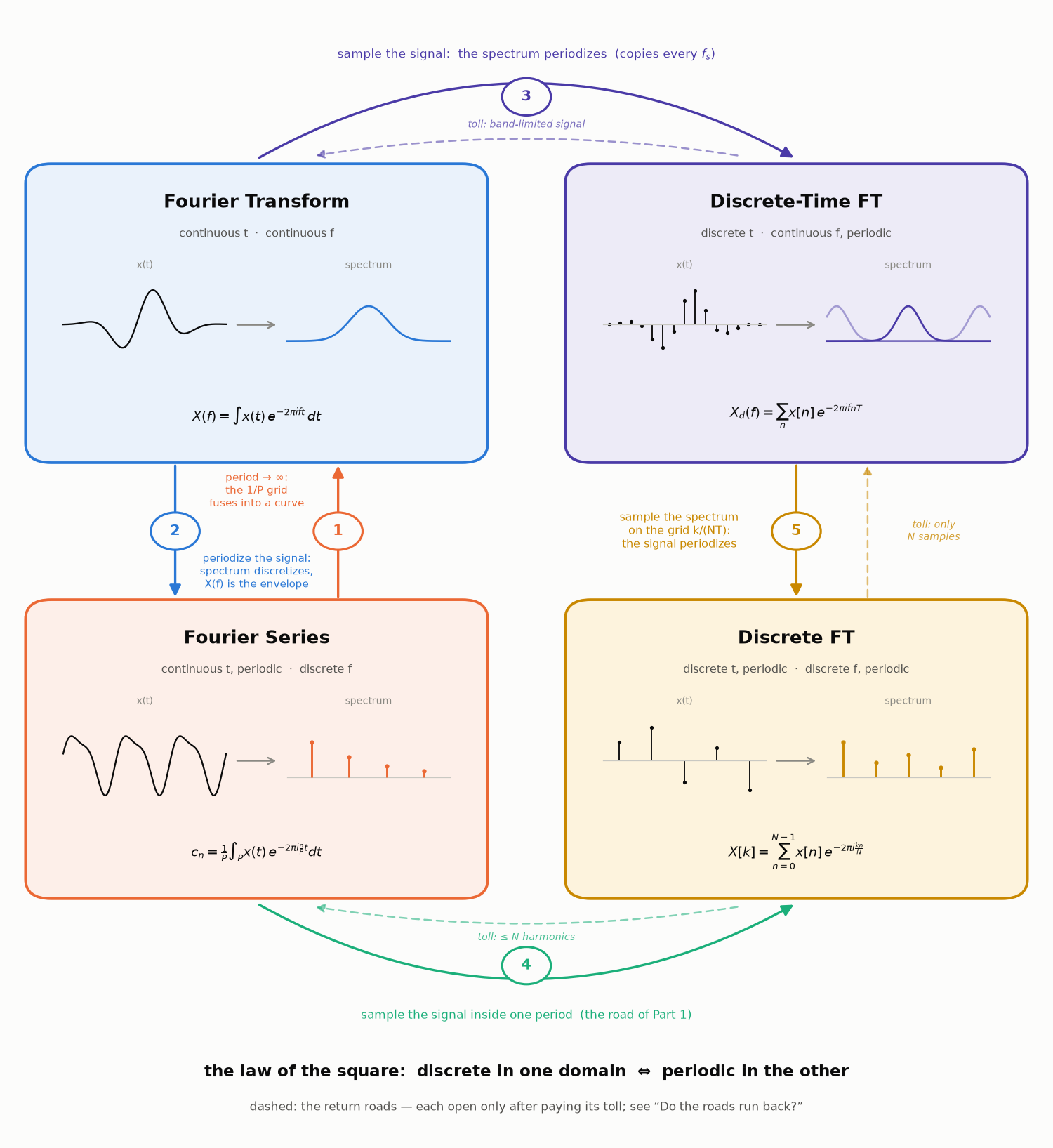
Two conventions carried over from the trilogy: frequencies live in hertz (the exponentials are $e^{\pm 2 \pi i f t}$, no loose $\omega$’s), and all the machinery for discrete signals — the delta function, the sifting property, the comb — is the one built honestly in Part 1; we will lean on it without re-deriving. And a calibration of rigor: most steps today are honest, and where the classical fine print matters we will say so and point to it. One physicist’s shortcut does remain, in bridge one: an approximation slips inside an infinite sum before the limit is taken. Part 1 shows what making such a step fully honest costs — we will flag it there and move on.

The cast, in one paragraph each

The Fourier series (Part 1’s workhorse): a periodic signal with period $P$ is a weighted sum of harmonics — frequencies $\frac{n}{P}$, a discrete grid with step $\frac{1}{P}$:

$$ x(t) = \sum_{n = -\infty}^{\infty} c_n\, e^{2 \pi i \frac{n}{P} t}, \qquad c_n = \frac{1}{P} \int_{-P/2}^{P/2} x(t)\, e^{-2 \pi i \frac{n}{P} t}\, dt. $$

Continuous periodic time, discrete frequency. The other three shades we will construct — from this one.

Bridge one: Fourier series → Fourier transform

The series serves periodic signals only. What about a signal that never repeats — a single pulse, a spoken sentence, anything from the real world? Call it a periodic signal whose period is infinite, and watch what happens to the machinery as $P$ grows:

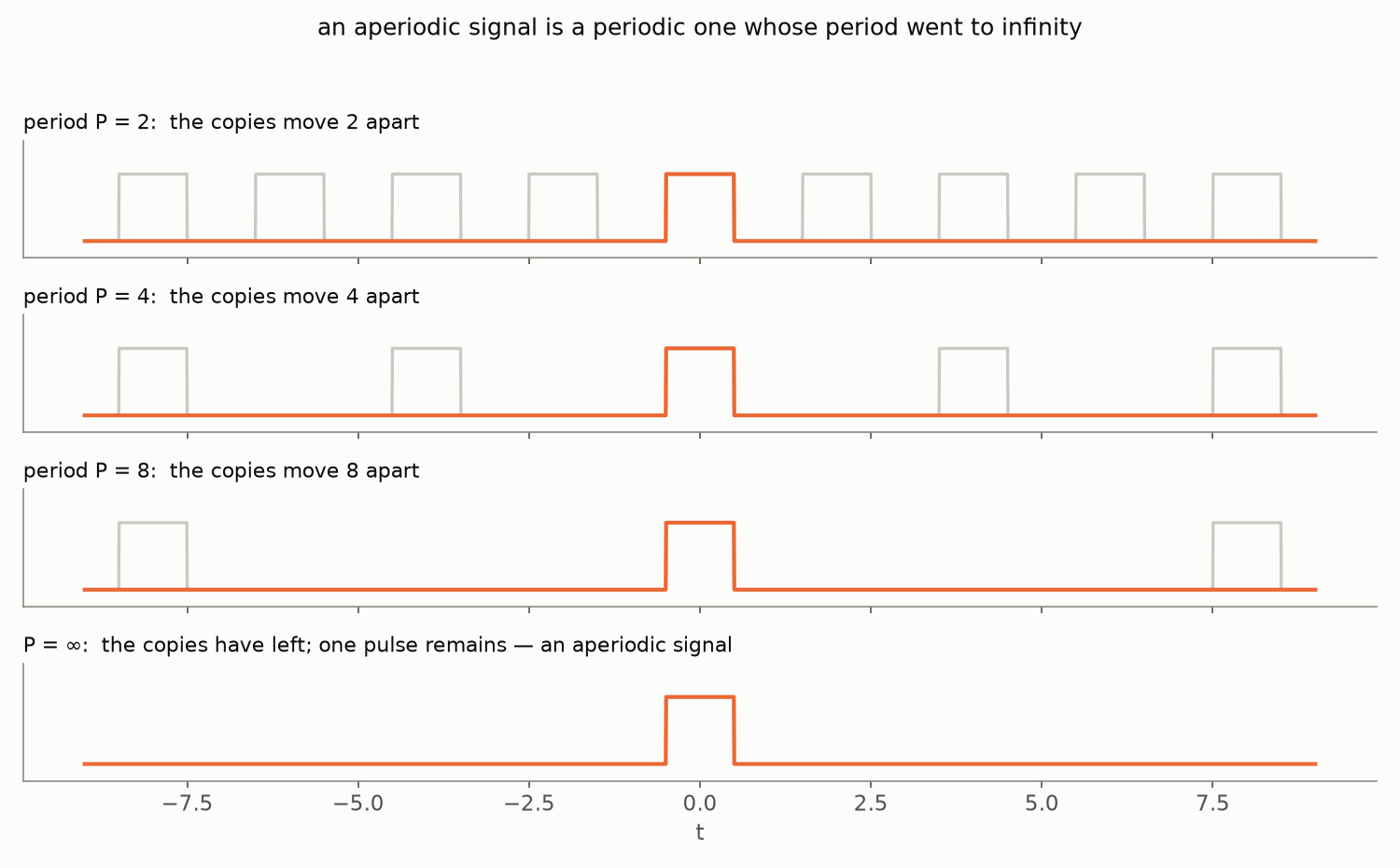
In the time domain the copies march off to infinity, leaving one pulse. In the frequency domain something more interesting happens. Rewrite the series, multiplying and dividing by $P$:

$$ x(t) = \sum_{n=-\infty}^{\infty} c_n\, e^{2 \pi i \frac{n}{P} t} = \sum_{n=-\infty}^{\infty} \left( c_n P \right) e^{2 \pi i f_n t} \cdot \frac{1}{P}, \qquad f_n = \frac{n}{P}. $$

The combination $c_n P$ is an integral that no longer hides a $\frac{1}{P}$:

$$ c_n P = \int_{-P/2}^{P/2} x(t)\, e^{-2 \pi i f_n t}\, dt. $$

As $P \to \infty$, the integration limits open up to the whole axis, and $c_n P$ approaches the value of one fixed function at the point $f_n$ — give it a name:

$$ X(f) = \int_{-\infty}^{\infty} x(t)\, e^{-2 \pi i f t}\, dt. $$

Now look at the sum we are left with:

$$ x(t) \approx \sum_{n=-\infty}^{\infty} X(f_n)\, e^{2 \pi i f_n t} \cdot \frac{1}{P} $$

This final sum is an integral sum — a Riemann sum, an old friend from Part 1 — for the function $X(f)\, e^{2 \pi i f t}$ over the partition $f_n$ of the frequency axis, whose norm is the difference of adjacent points: $f_{n+1} - f_n = \frac{1}{P}$. As $P \to \infty$, the norm of the partition goes to $0$, and the sum converges to the integral:

$$ x(t) = \int_{-\infty}^{\infty} X(f)\, e^{2 \pi i f t}\, df $$

(understood as a symmetric limit of the integration bounds — the Cauchy principal value; more on this in a moment).

Meet the second shade. $X(f)$ is the Fourier transform of $x(t)$, and the last formula — the Fourier integral — is its inversion: the signal reassembled from a continuum of frequencies. Everything is as in the series, with the sum over a discrete grid of harmonics matured into an integral over all frequencies, and the coefficients $c_n$ matured into a density $X(f)$ (per unit of frequency — that is what the extra $P$ was doing).

Two remarks on honesty (when the principal value actually matters)

Formally, both integrals are defined with the symmetric-limit — principal-value — reading, and for a good reason: the definition must make sense even for inputs that are not absolutely integrable, and the inversion integral will need exactly that generosity. The real distinction between the two is when the principal value has actual work to do. Feed the forward transform an absolutely integrable signal — our standing assumption — and the caution turns out to be vacuous: $\left| x(t)\, e^{-2 \pi i f t} \right| = |x(t)|$, the integral converges absolutely, and every reasonable reading of it agrees. The inversion integral enjoys no such luck. Its input is $X$ — and $X$ need not be absolutely integrable even when $x$ was: our rectangular pulse’s transform will turn out to be a sinc, with tails dying like $\frac{1}{f}$ — too slowly (we compute it in bridge two). So there the principal value genuinely earns its keep. The inversion theorem pins down exactly when the symmetric limit returns $x(t)$ — under far weaker assumptions than our physicist’s derivation used. This is precisely how Zorich’s Mathematical Analysis II sets things up on p. 524 of the 9th Russian edition: both definitions carry the principal-value clause, and the absolute-convergence remark follows immediately for integrable inputs.

Bridge two: Fourier transform → Fourier series

Now walk the same bridge in the opposite direction — it reveals something the limit hid. Take an aperiodic signal $x(t)$ of finite extent (finite support, in the math vocabulary): zero outside $\left[ -\frac{\tau}{2}, \frac{\tau}{2} \right]$. It has a Fourier transform $X(f)$. Pick a period $P$ at least as large as the support, $P \ge \tau$, and copy the signal every $P$: this gives the periodic extension $x_P(t)$ — Part 1’s gluing again — and the copies never overlap:

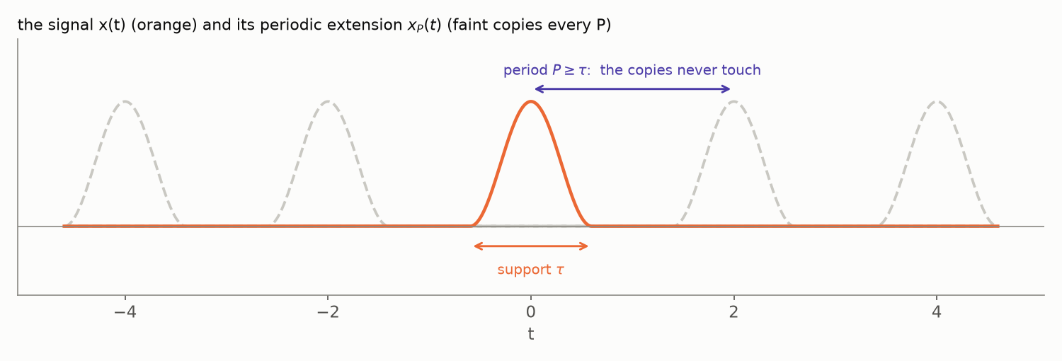
The extension is periodic, so it has a Fourier series; compute its coefficients:

$$ c_n = \frac{1}{P} \int_{-P/2}^{P/2} x_P(t)\, e^{-2 \pi i \frac{n}{P} t}\, dt = \frac{1}{P} \int_{-\infty}^{\infty} x(t)\, e^{-2 \pi i \frac{n}{P} t}\, dt $$

— inside one period, $x_P$ is $x$ (the other copies live outside), so the finite integral quietly unfolds into the infinite one. But the right-hand side is the Fourier transform of $x$, evaluated at $f_n = \frac{n}{P}$:

$$ c_n = \frac{1}{P}\, X\!\left( \frac{n}{P} \right). $$

Read it as a picture: the Fourier coefficients of the periodized signal are samples of one continuous curve — the transform $\frac{1}{P} X(f)$ is the envelope of the discrete spectrum. Make the period longer, and the samples pack tighter along the same envelope, until they fuse into it:

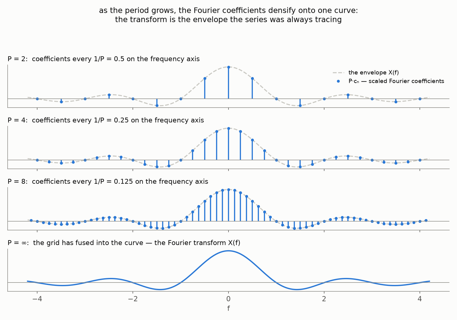
(The stems in the picture are drawn as $P \cdot c_n$ — the raw coefficients themselves shrink like $\frac{1}{P}$ and would sink into the axis; the shape is what survives, and the shape is $X(f)$.)

And what is that envelope, for the rectangular pulse of the pictures? For once, a transform we can compute end to end — the pulse has height $1$ on $\left[ -\frac{1}{2}, \frac{1}{2} \right]$, so:

$$ \begin{aligned} X(f) = \int_{-1/2}^{1/2} e^{-2 \pi i f t}\, dt &= \left. \frac{e^{-2 \pi i f t}}{-2 \pi i f} \right|_{t=-1/2}^{t=1/2} \\ &= \frac{e^{\pi i f} - e^{-\pi i f}}{2 \pi i f} = \frac{\sin(\pi f)}{\pi f}, \end{aligned} $$

the last step being Euler’s formula run backwards, $\sin z = \frac{1}{2i} \left( e^{iz} - e^{-iz} \right)$. This damped ripple is the sinc function. Look back at the envelope figure: the tips of the stems lie exactly on this curve — sinc is the envelope the coefficients were densifying onto. And it is the promised troublemaker of bridge one: its tails die like $\frac{1}{f}$, too slowly for absolute integrability, which is exactly why the inversion integral keeps its principal-value clause.

This bridge also plants the law that will organize everything below. Periodizing the signal made its spectrum discrete — samples on the grid $\frac{n}{P}$. Periodic in time ⇔ discrete in frequency, and the period in one domain sets the grid step in the other: $P$ seconds of period — $\frac{1}{P}$ hertz between harmonics. The bridge we have just crossed is the left edge of our map — and by the end of this post the same law will run every road on it.

Bridge three: Fourier transform → DTFT

So far both shades live on continuous time. Enter the sampled world — through the honest gate built in Part 1: a discrete signal is the analog signal times the comb, $x_d(t) = x(t) \cdot \text{Ш}_T(t) = \sum_n x(nT)\, \delta(t - nT)$. One thing is genuinely new here. In Part 1 every integral ran over a bounded stretch — a neighborhood of one sampling point, a single period — so only finitely many teeth of the comb ever fell inside. The transform integral runs over the whole line, and for the first time all the teeth speak at once. So truncate the train for a moment — keep only the samples with $|n| \le N$ — and transform this finite piece, step by step:

$$ \begin{aligned} \int_{-\infty}^{\infty} \left( \sum_{n=-N}^{N} x(nT)\, \delta(t - nT) \right) e^{-2 \pi i f t}\, dt &= \sum_{n=-N}^{N} x(nT) \int_{-\infty}^{\infty} \delta(t - nT)\, e^{-2 \pi i f t}\, dt \\ &= \sum_{n=-N}^{N} x(nT)\, e^{-2 \pi i f n T}. \end{aligned} $$

Both moves are fully covered by Part 1’s machinery: a finite sum crosses the integral by plain linearity, and then the sifting property proved in Part 1 collapses each integral — every delta samples the exponential at its own grid instant $t = nT$.

The full train is the $N \to \infty$ limit of its truncations,

$$ x_d(t) = \lim_{N \to \infty} \sum_{n=-N}^{N} x(nT)\, \delta(t - nT), $$

so we define its transform as the limit of the finite results:

$$ X_d(f) \;\overset{\text{def}}{=}\; \lim_{N \to \infty} \sum_{n=-N}^{N} x(nT)\, e^{-2 \pi i f n T} = \sum_{n=-\infty}^{\infty} x(nT)\, e^{-2 \pi i f n T}, $$

asking, as is only fair for a definition-by-limit, that the limit exist. A clean sufficient condition: the samples are absolutely summable, $\sum_n |x(nT)| \lt \infty$. Each term of our series has absolute value $|x(nT)|$ — the exponential contributes only a phase — so by the Weierstrass M-test the series then converges at every $f$, and uniformly at that.

The textbook reference (chapter and page in Oppenheim & Schafer)

This is also exactly how the standard textbook introduces the object. Oppenheim & Schafer’s classic Discrete-Time Signal Processing (3rd edition, Pearson New International Edition, Pearson 2014; ch. 2, “Discrete-Time Signals and Systems”, §7 “Representation of Sequences by Fourier Transforms”, pp. 50–52) defines the transform as the limit of precisely our symmetric truncations — their Eq. (134) — and reaches absolute summability as the sufficient condition for uniform convergence through the same bound.

Before naming it, notice its defining feature. Shift $f$ by $f_s = \frac{1}{T}$: each term picks up $e^{-2 \pi i n} = 1$ — nothing changes. The spectrum of a sampled signal is periodic with period $f_s$ — and the reason is, once again, that $n$ is an integer: sampling put the signal on a grid, and a whole number of extra turns changes no exponential. It is the same one-line argument that gave $c_{k+N} = c_k$ in Part 1, now acting in the other domain. Set the notational convention $T = 1$ (indices instead of seconds, square brackets as in Part 1) and this sum is the third shade, the discrete-time Fourier transform:

$$ X_d(f) = \sum_{n=-\infty}^{\infty} x[n]\, e^{-2 \pi i f n} $$

— discrete time in, continuous (and periodic) frequency out. The mirror image of the Fourier series, cell for cell: there, continuous periodic time and discrete frequency; here, discrete time and continuous periodic frequency.

The copies: what sampling does to a spectrum

Periodicity is only half the story. The other half is what exactly one period of $X_d$ contains — and here bridge two pays an unexpected dividend: its envelope formula, $c_n = \frac{1}{P} X\!\left(\frac{n}{P}\right)$, is about to be reused with the roles of time and frequency swapped. Consider the periodization of the original spectrum $X(f)$ along the frequency axis, copies every $f_s$:

$$ Y(f) = \sum_{m=-\infty}^{\infty} X(f - m f_s). $$

$Y$ is $f_s$-periodic, so it expands in a Fourier series in the frequency variable — the harmonics are $e^{-2 \pi i f n T}$, indexed by time lags $nT$. Compute its coefficients:

$$ d_n = \frac{1}{f_s} \int_{-f_s/2}^{f_s/2} Y(f)\, e^{2 \pi i f n T}\, df = \frac{1}{f_s} \int_{-\infty}^{\infty} X(f)\, e^{2 \pi i f n T}\, df = \frac{1}{f_s}\, x(nT). $$

Two transitions here: 1) the integral of a periodization over one period equals the integral of the original over the whole line — bridge two’s unfolding trick, and the harmonic rides along untouched because it is itself $f_s$-periodic; 2) the middle expression is the Fourier inversion integral of bridge one, evaluated at $t = nT$ — it reassembles the sample $x(nT)$.

So the periodized spectrum is $Y(f) = \sum_n \frac{x(nT)}{f_s} e^{-2 \pi i f n T} = T \cdot X_d(f)$, that is:

$$ X_d(f) = \frac{1}{T} \sum_{m=-\infty}^{\infty} X(f - m f_s). $$

The DTFT is the original transform, copied every $f_s$ and stacked. Sampling in time periodizes the spectrum — the exact dual of bridge two, proved by bridge two, run in the other domain. (Mathematicians know this identity as the Poisson summation formula; we got it by crossing our own bridge twice. To see the match, set $f = 0$: the copies formula collapses to the textbook statement $\sum_n x(nT) = \frac{1}{T} \sum_m X(m f_s)$ — the sum of a signal’s samples equals, up to $\frac{1}{T}$, the sum of its spectrum’s samples.)

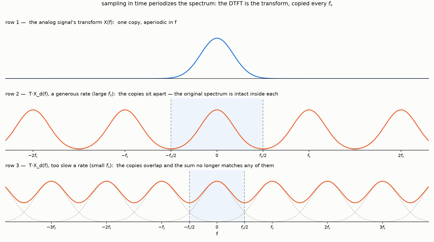
The picture holds a loaded gun. If the copies don’t reach each other — if $X(f)$ lives entirely below $\frac{f_s}{2}$ — then one period of the DTFT contains an intact, undamaged copy of $X$: nothing about the analog signal was lost by sampling it. Cut that copy out, run the Fourier integral, and the continuous signal comes back — every value between the samples included. That is precisely the sampling theorem stated in Part 2 — and row 2 of the picture above is its proof, one post away from being written out. If the copies do overlap (row 3), they add up where they collide, and no cutting recovers $X$ — aliasing, the theorem’s dark twin, again exactly as promised.

Bridge four: Fourier series → DFT

The fourth shade needs no new work at all: it is the road Part 1 walked end to end — the bottom edge of the map. Take $N$ samples, periodize with period $NT$, feed the comb into the Fourier series, let sifting collapse the integral:

$$ c_k = \frac{1}{NT} \sum_{n=0}^{N-1} x(nT)\, e^{-2 \pi i \frac{k n}{N}}, $$

$T$ cancels in the exponent, only $N$ coefficients are distinct, and dropping the physical scale leaves the discrete Fourier transform $X[k] = \sum_n x[n]\, e^{-2 \pi i k n / N}$ — discrete and periodic in both domains, the fully quantized corner of the table.

Note that this one road makes two moves at once — it samples the signal, and it periodizes it — so both faces of the law fire together. The sampling made the spectrum periodic: one line, $c_{k+N} = c_k$. The periodization made the spectrum discrete: a Fourier series hands over coefficients on a grid by its very construction. This is where Part 2 of the spectrogram series, Reading the DFT, first met both faces of the law — by direct computation, before any general principle was in sight.

Bridge five: DTFT → DFT

One connection remains: the two discrete-time shades. The DTFT of a finite recording ($x[n] = 0$ outside $0, \dots, N-1$) is a continuous periodic curve; the DFT is $N$ numbers. Evaluate the DTFT on the grid $f_k = \frac{k}{NT}$ — $N$ points per period — and compare:

$$ X_d\!\left( \frac{k}{NT} \right) = \sum_{n=0}^{N-1} x(nT)\, e^{-2 \pi i \frac{k}{NT} n T} = \sum_{n=0}^{N-1} x[n]\, e^{-2 \pi i \frac{k n}{N}} = X[k]. $$

The DFT bins are samples of the DTFT — no new transform, just $N$ readings of the continuous curve:

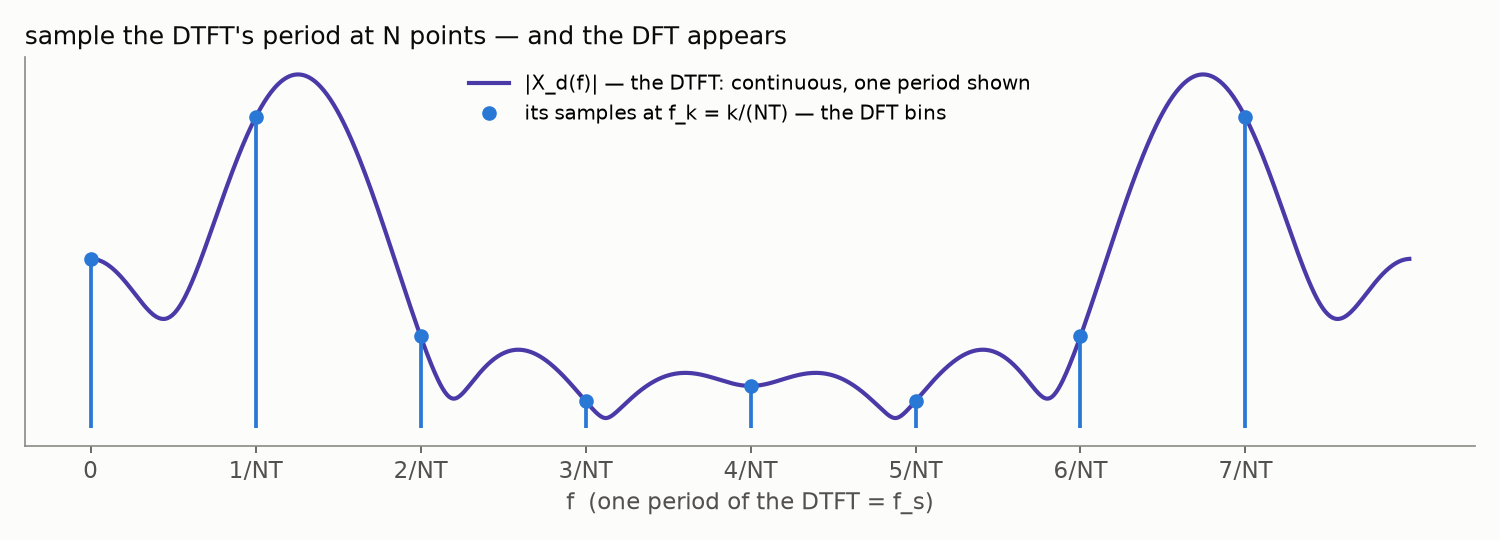
And the law completes its square. What did we pay for making the spectrum discrete? Look back at bridge four: the price was periodizing the signal — the glued copies. Sampling the spectrum periodizes the signal, exactly as sampling the signal periodized the spectrum. Part 2 even drew what that costs: the DFT’s model of a signal repeats forever with the window’s period — that repetition is the time-domain periodization that bridge five smuggles in. (Bridges four and five agree to the letter: $c_k = \frac{1}{NT} X_d(f_k)$ — the envelope relation of bridge two, one floor down the table.)

Do the roads run back?

Look at the arrows: every one of them points toward discreteness. The DFT is a sink — three roads lead in, none lead out. Is the traffic really one-way?

For arbitrary signals, yes. Sampling discards everything between the samples; periodizing overlaps everything that pokes out of one period. A general crossing loses information, and lost information buys no return ticket. But each bridge does have a return ticket, and all the tickets carry the same fine print: a crossing is reversible exactly when the other domain is limited.

• DFT → DTFT. If the signal is time-limited to $N$ samples, the continuous curve $X_d(f)$ is completely determined by its $N$ readings. The argument (Oppenheim & Schafer, ch. 8, §4 “Sampling the Fourier Transform”, pp. 666–669) is bridge five’s law once more: keep only $N$ readings of the curve, and the time signal they encode is not $x[n]$ but its periodization $\sum_r x[n - rN]$ — sampling in frequency periodizes time. A signal that lives on $N$ samples fits inside one period, so the copies do not overlap and an intact $x$ sits in each: copy those $N$ samples out of one period, plug them into the sum $X_d(f) = \sum_n x[n]\, e^{-2 \pi i f n T}$, and the curve is back — computable at every frequency. (The explicit interpolation formula that does all of this in one step is their Problem 57.) But the toll is real, and it is charged daily: when the $N$ samples are a window cut from a longer signal — every frame of Part 3’s spectrograms — the road leads back to the DTFT of the window, not of the signal, and the gap between the two is exactly the leakage Part 3 measured. For a discrete signal stretching over the whole time axis, no finite batch of readings pins the curve down at all.
• DFT → FS. If a periodic signal contains only $N$ harmonics, its $N$ coefficients rebuild it exactly — this is the trigonometric interpolation of Part 2’s green model, the curve through every sample.
• DTFT → FT. The copies picture already said it: if the signal was band-limited below $\frac{f_s}{2}$, the copies never touch, and one period of the DTFT holds an intact $X(f)$ — cut it out, and the transform (hence the signal, every value between the samples included) is recovered. That return ticket is the sampling theorem of Kotelnikov–Shannon–Nyquist, and its price — band-limitedness — is precisely the fine print the next post will read aloud.

So the law of the square has a quieter second half: limited in one domain ⇔ recoverable from samples in the other. Sampling time costs nothing when the frequency content is limited; sampling frequency costs nothing when the time extent is limited. The DFT sits in its corner not as a grave but as a compressed archive.

(One caveat for the perfectionist: the full journey back — DFT all the way to the analog world — needs time-limitedness and band-limitedness at once, and a nonzero signal cannot strictly have both. The round trip to the analog world is therefore always an approximation; how good an approximation is, once again, the sampling theorem’s department.)

Why can't a signal be time-limited and band-limited at once? (a Taylor series settles it)

Suppose $x$ is band-limited: $x(t) = \int_{-B}^{B} X(f)\, e^{2 \pi i f t}\, df$, an integral over a finite stretch of frequencies. Differentiate under the integral as many times as you like — each derivative pulls down one factor of $2 \pi i f$, and $|f| \le B$ caps it:

$$ \left| x^{(k)}(t) \right| \le (2 \pi B)^k \int_{-B}^{B} |X(f)|\, df = C \cdot (2 \pi B)^k. $$

The derivatives grow at most geometrically — and a factorial beats any geometric growth. Two small gears turn inside that claim, so let us expose them. First, the Lagrange form of the Taylor remainder: cutting the Taylor series of $x$ around $t_0$ after $k$ terms leaves the error

$$ R_k(t) = \frac{x^{(k+1)}(\xi)}{(k+1)!}\, (t - t_0)^{k+1} \quad \text{for some } \xi \text{ between } t_0 \text{ and } t, $$

so the error is controlled by the next derivative, and our bound turns it into $|R_k(t)| \le C\, \frac{a^{k+1}}{(k+1)!}$ with $a = 2 \pi B\, |t - t_0|$ — a fixed number once $t$ is fixed. Second, why does $\frac{a^k}{k!}$ go to $0$? Compare successive terms: the ratio is $\frac{a}{k+1}$, which drops below $\frac{1}{2}$ as soon as $k$ passes $2a$ — from that point on every term at least halves. The factorial outruns any geometric growth; this is the same reason the series for $e^{z}$ converges everywhere. And “the remainder tends to zero” is literally the statement “the Taylor series converges to $x(t)$”: the remainder is, by definition, the gap between $x(t)$ and the first $k$ terms. A band-limited signal is, in other words, an analytic function — and of the strongest kind. Look at what the bound delivered: $a = 2 \pi B\, |t - t_0|$ is finite for every $t$, however far from $t_0$, so the Taylor series around any single point converges to $x$ on the whole line — the radius of convergence is infinite (in complex-analysis vocabulary, $x$ extends to an entire function). And a power series leaves no freedom: inside its radius of convergence the coefficients are forced — they can only be $\frac{x^{(k)}(t_0)}{k!}$. So the behavior of $x$ on any tiny interval around $t_0$, which already pins down all the derivatives there, pins down $x$ everywhere. (Part 1’s “why not Taylor?” inset complained that Taylor coefficients are rigidly global creatures — here, at last, that rigidity does useful work.)

Now let $x$ also be time-limited: identically zero outside some interval. Pick $t_0$ in the silence. Every derivative of $x$ at $t_0$ is zero, so the Taylor series is the zero series — and by the paragraph above it converges to $x$ everywhere. Hence $x \equiv 0$. A signal that is not identically zero must overflow either its time box or its frequency box.

The map, walked

Here is the same map from the top of the post once more — only now every road on it has been built underfoot:

One law runs every road: discrete in one domain ⇔ periodic in the other — and quantitatively, a period of $A$ in one domain forces a grid of step $\frac{1}{A}$ in the other. Sample a signal every $T$ seconds, and its spectrum repeats every $\frac{1}{T}$ hertz. Periodize a signal every $P$ seconds, and its spectrum collapses to the grid $\frac{n}{P}$. Do both — which is what any computer holding $N$ samples has silently done — and both domains end up discrete and periodic: the DFT, with its $N$-point grids locked in the relation $\Delta f = \frac{1}{NT}$ that Part 2 spent a whole section reading.

The square also says what comes next. Row 2 of the copies picture from bridge three — separated copies, the original spectrum intact inside each — is the entire proof of the theorem with three names, waiting to be written carefully: what “band-limited” must mean, why the boundary case bites, how the sinc reconstructs, and what the wagon wheels in old westerns have to do with any of it. The theorem’s post is next on this road.